1.2. Activation Functions

Activation functions are essential components of artificial neural networks, and modern architectures—such as convolutional neural networks (CNNs) and vision transformers (ViTs)—use them extensively across various data domains. Activation functions bring several benefits:

1. Stabilising the optimisation process: Many activation functions restrict output values to a finite range, which can help keep the network’s behaviour stable during training.

2. Adding non-linearity: Like complex cells in the visual cortex that cannot be represented by simple linear operations, artificial neural networks also rely on non-linear activation functions to solve non-linear problems. These functions enable the network to learn complex patterns in the data.

Most activation functions operate on each element of the input independently—known as elementwise operations. PyTorch provides a variety of non-linear activation functions, which you can explore in their documentation.

0. Preparation

Before we dive into the main content of this notebook, let’s start by preparing all the necessary materials.

Required Packages

We will need several libraries to implement this tutorial, each serving a specific purpose:

• numpy: The main package for scientific computing in Python. It’s commonly imported with the alias np to simplify its use in code.

• matplotlib: A library for plotting graphs and visualising data in Python.

• torch: A deep learning framework that helps us define neural networks, manage datasets, optimise loss functions, and more.

# Importing the necessary libraries
import numpy as np
from matplotlib import pyplot as plt
import torch

Input tensor

For this notebook, we’ll use an input tensor ranging from \(-10\) to \(10\) to explore how different activation functions respond to various input values.

# Creating a tensor with values ranging from -10 to 10
input_tensor = torch.arange(-10, 11).float()
print("Input tensor:", input_tensor)

Input tensor: tensor([-10.,  -9.,  -8.,  -7.,  -6.,  -5.,  -4.,  -3.,  -2.,  -1.,   0.,   1.,
          2.,   3.,   4.,   5.,   6.,   7.,   8.,   9.,  10.])

1. ReLU (Rectified Linear Unit)

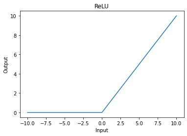
ReLU (Rectified Linear Unit) is one of the most popular activation functions. It’s defined as:

\(ReLU(x)=(x)^+=max(0,x)\)

This function sets any negative values to zero, allowing only positive values to pass through. ReLU introduces non-linearity to the network while keeping computations efficient.

# Initialising the ReLU activation function
relu = torch.nn.ReLU()

# Plotting ReLU to visualise its behaviour
plt.plot(input_tensor, relu(input_tensor))
plt.xlabel('Input')
plt.ylabel('Output')
plt.title("ReLU")
plt.show()

2. Other Non-linear Functions

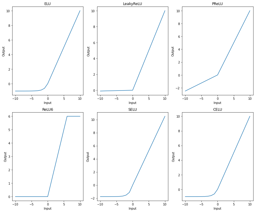
Now, let’s explore a variety of other non-linear activation functions in PyTorch. Each activation function has unique properties and behaviours. Here, we will plot a selection of functions and examine their outputs across our input tensor.

We define several popular non-linear functions in a dictionary and iterate over them to plot each one:

# Defining a dictionary of different non-linear activation functions
non_linear_funs = {
    'ELU': torch.nn.ELU(),         # Exponential Linear Unit
    'LeakyReLU': torch.nn.LeakyReLU(), # Allows a small gradient when input is negative
    'PReLU': torch.nn.PReLU(),     # Parametric ReLU with learnable parameter for the slope
    'ReLU6': torch.nn.ReLU6(),     # ReLU with an upper limit at 6
    'SELU': torch.nn.SELU(),       # Scaled ELU, which maintains a self-normalising effect
    'CELU': torch.nn.CELU(),       # Continuously Differentiable ELU
}

# Setting up a figure to plot each activation function’s behaviour
fig = plt.figure(figsize=(12, 10))
for i, (name, fun) in enumerate(non_linear_funs.items()):
    ax = fig.add_subplot(2, 3, i+1)
    # Applying the activation function and plotting its output
    ax.plot(input_tensor, fun(input_tensor).detach().numpy())
    ax.set_title(name)  # Title of the plot is the function's name
    ax.set_xlabel('Input')
    ax.set_ylabel('Output')

plt.tight_layout()
plt.show()

In this visualisation:

• Each subplot represents one of the activation functions, showing its effect across the input range.

• Note how different functions handle negative values and how some functions have upper limits on the output, which can impact the overall behaviour of the network. For example:

  • ELU gradually allows negative values, avoiding sharp transitions.

  • LeakyReLU introduces a small slope for negative values, allowing some gradient flow even when inputs are negative.

  • ReLU6 has an upper limit, restricting the output to the range \([0, 6]\).

These unique characteristics allow you to choose the most appropriate activation function based on the network’s needs and the nature of the data.