5.2. Text Classification#
In this notebook, we will learn how to perform a simple text classification using torchtext. This is similar to the image classification problem, in which the network’s task is to assign a label to the given image but in text.
Text data is more like an audio signal in terms of its dimensionality (i.e., 1D). They are both a sequence of numbers:
In an audio signal the sequence is temporal.
In the text data the sequence is positional (i.e., the position of words in a sentence).
0. Preparation#
In order to run this notebook, we need to perform some preparations.
We use datasets from torchtext that require portalocker package.
In Google Colab you can install it by uncommenting and executing the next
code cell.
# !pip install portalocker>=2.0.0
Packages#
Let’s start with all the necessary packages to implement this tutorial.
numpy is the main package for scientific computing with Python. It’s often imported with the
npshortcut.termcolor is an ANSI colour formatting for output in the terminal.
matplotlib is a library to plot graphs in Python.
os provides a portable way of using operating system-dependent functionality, e.g., modifying files/folders.
torch is a deep learning framework that allows us to define networks, handle datasets, optimise a loss function, etc.
import numpy as np
import os

from matplotlib import pyplot as plt
from termcolor import colored

import torch
import torch.nn as nn
import torchtext
Device#
Choosing CPU or GPU based on the availability of the hardware.
device = torch.device('cuda' if torch.cuda.is_available() else 'cpu')
print('Selected device:', colored(device, 'red'))
Selected device: cuda
1. Dataset#
The torchtext.dataset offers easy access to several text datasets. In this tutorial, we use the AG’s News Corpus dataset that contains 120000 samples for training and 7600 for testing. Each piece of news corresponds to one of the following four categories:
World
Sport
Business
Sci/Tec
To load our dataset:
We use the
torchtext.datasets.AG_NEWSmodule.The first time you execute the next cell, it downloads the dataset and extracts its content in the
./data/directory.torchtextdatasets are implemented in an iterable-style unliketorchvision/torchaudiowhich are map-style. So we call theto_map_style_datasetto convert the dataset into map-style. This way we can reuse a large part of our training/testing pipeline from image/audio classification notebooks.
train_db = torchtext.datasets.AG_NEWS(root='./data/', split="train")
test_db = torchtext.datasets.AG_NEWS(root='./data/', split="test")

train_db = torchtext.data.functional.to_map_style_dataset(train_db)
test_db = torchtext.data.functional.to_map_style_dataset(test_db)
We create a dict to convert label numbers to human-readable text. Please note that in
Python indexing starts from 0 therefore the labels are in the range of 0-3 (the raw data
in the downloaded CSV files is in the range of 1-4)-
ag_news_labels = {
    0: "World",
    1: "Sports",
    2: "Business",
    3: "Sci/Tec"
}
Let’s get one sample from our dataset and print its content:
label_sample, text_sample = train_db.__getitem__(0)
print(label_sample, ag_news_labels[label_sample-1])
print(text_sample)
3 Business
Wall St. Bears Claw Back Into the Black (Reuters) Reuters - Short-sellers, Wall Street's dwindling\band of ultra-cynics, are seeing green again.
Preprocessing#
The news piece in the raw data is in the form of a string. We should process this into an array of numbers before passing it to a network. This consists of the following steps:
Splitting the text (string sentence) into the smallest units (tokens).
Creating a dictionary (i.e., look up table) of all words (tokens) in our dataset.
We convert the raw text into indices of this dictionary.
Tokeniser#
We simply use the get_tokenizer function to split the text into the smallest units (tokens).
Our dataset is in English therefore we pass the basic_english which defines how to tokenise
a string (e.g., by words, spaces and punctuations).
tokeniser = torchtext.data.utils.get_tokenizer("basic_english")
Let’s use the tokenise with one sample from our dataset to inspect its output.
tokned_string = tokeniser(text_sample)
print('The string consists of %d tokens:\n%s' % (len(tokned_string), tokned_string))
The string consists of 29 tokens:
['wall', 'st', '.', 'bears', 'claw', 'back', 'into', 'the', 'black', '(', 'reuters', ')', 'reuters', '-', 'short-sellers', ',', 'wall', 'street', "'", 's', 'dwindling\\band', 'of', 'ultra-cynics', ',', 'are', 'seeing', 'green', 'again', '.']
Vocabulary#
We use the torchtext.vocab.build_vocab_from_iterator to create the dictionary for our dataset:
The first argument is an iterator. We create the
tokens_iterfunction which simply iterates over the entire dataset andyieldthe tokenised text.In the second argument we can pass a list of special characters. In this case, we only pass
"<unk>"(out-of-vocabulary or unknown word).Finally, by calling the
set_default_indexwe specify that if a word (token) in a sentence doesn’t exist in the vocabulary, assign it to the"<unk>"token.
def tokens_iter(dataset):
    for i in range(dataset.__len__()):
        _label, text = dataset.__getitem__(i)
        yield tokeniser(text)

db_vocab = torchtext.vocab.build_vocab_from_iterator(tokens_iter(train_db), specials=["<unk>"])
db_vocab.set_default_index(db_vocab["<unk>"])
Let’s have a look at the number of words in our dictrionary.
print('The number of words in the dictrionary: %d' % len(db_vocab))
The number of words in the dictrionary: 95811
Let’s print the first ten words (tokens) in our dataset:
ten_tokens = db_vocab.lookup_tokens(np.arange(10))
for tind, token in enumerate(ten_tokens):
    print('%d: %s' % (tind, token))
0: <unk>
1: .
2: the
3: ,
4: to
5: a
6: of
7: in
8: and
9: s
Raw-text to dictionary-index#
We create rawtex2dicind which is a small anonymous function (lambda) that converts the raw-text into dictionary-indices.
rawtex2dicind = lambda x: db_vocab(tokeniser(x))
Let’s call the dictrionary with a small sentence to check what is its output.
rawtex2dicind('This is a jupyter notebook.')
[52, 21, 5, 0, 1928, 1]
The output is the index of tokens (words) in our dictionary. We already knew the index of:
“a”: 5
“jupyter”: 0 because it’s unknown
“.”: 1
Note, that the dictrionary is case insensitive. There “a” and “A” result in the same index.
Dataloaders#
The length of sentences differs for each sample. This would cause an issue in creating the batch data (i.e., several texts). To create a tensor variable, all elements must have the same size. To overcome this, we pad the texts (i.e., the output of rawtex2dicind) with zeros to equalise all audio samples in a batch. This is implemented as follows:
We create “custom” batches by passing
collate_fn=collate_fntotorch.utils.data.DataLoader(for more details check its documentation).We implement the
collate_fnthat calls therawtex2dicindfunction.We pass the texts to
pad_sequencewhich makes them of identical size.
def pad_sequence(batch):
    # Make all tensor in a batch the same length by padding with zeros
    # for item in batch:
    #     print(len(item))
    batch = [item.t() for item in batch]
    batch = torch.nn.utils.rnn.pad_sequence(batch, batch_first=True, padding_value=0)
    # print(batch.shape)
    return batch

def collate_fn(batch):
    texts, targets = [], []
    for label_b, text_b in batch:
        # we tokenise it, get the vocabulary index and convert it to tensor
        texts.append(torch.tensor(rawtex2dicind(text_b), dtype=torch.int64))
        targets.append(int(label_b) - 1)  # -1 to bring label to 0 (the raw data start from 1)
    texts = pad_sequence(texts)
    # print(targets)
    targets = torch.tensor(targets)
    return texts, targets

train_loader = torch.utils.data.DataLoader(
    train_db, batch_size=128, shuffle=True, collate_fn=collate_fn
)

test_loader = torch.utils.data.DataLoader(
    test_db, batch_size=32, shuffle=False, collate_fn=collate_fn
)
2. Network#
We define our network in the class TextClassificationNet. It consists of two layers:
nn.EmbeddingBagto compute features. An EmbedingBag layer computes sums/means of “bags” of embeddings, without instantiating the intermediate embeddings. In our example, the number of embeddings is the number of words in our vocabulary. When we pass a text to this layer, it uses the values corresponding to the bags (indices) of those existing within the text.nn.Linear: standard classification layer.
Usually, more advanced transforms are applied to the text data, however, this is beyond the scope of this notebook and the text classification we want to solve here.
class TextClassificationNet(nn.Module):
    def __init__(self, vocab_size, embed_dim, num_class):
        super(TextClassificationNet, self).__init__()
        self.embedding = nn.EmbeddingBag(vocab_size, embed_dim, sparse=False)
        self.fc = nn.Linear(embed_dim, num_class)

    def forward(self, text):
        embedded = self.embedding(text)
        return self.fc(embedded)
Let’s make an instance of this model and print it’s parameters.
num_classes = len(set([label for (label, text) in train_db]))
vocab_size = len(db_vocab)
emb_size = 64
model = TextClassificationNet(vocab_size, emb_size, num_classes).to(device)
print(model)

def count_parameters(model):
    return sum(p.numel() for p in model.parameters() if p.requires_grad)

num_model_parameters = count_parameters(model)
print("Number of parameters: %s" % num_model_parameters)
TextClassificationNet(
  (embedding): EmbeddingBag(95811, 64, mode='mean')
  (fc): Linear(in_features=64, out_features=4, bias=True)
)
Number of parameters: 6132164
3. Train/test routines#
The following routines are very similar (close to identical) to what we previously saw in the image/audio classification problem we have seen previously.
def epoch_loop(model, dataloader, criterion, optimiser, log_frequency=5000):
    # usually the code for train/test has a large overlap.
    is_train = False if optimiser is None else True

    # model should be in train/eval model accordingly
    model.train() if is_train else model.eval()

    accuracies = []
    losses = []
    with torch.set_grad_enabled(is_train):
        for batch_ind, (text, target) in enumerate(dataloader):
            text = text.to(device)
            target = target.to(device)

            output = model(text)
            # computing the loss
            loss = criterion(output, target)
            # torch.nn.utils.clip_grad_norm_(model.parameters(), 0.1)
            losses.extend([loss.item() for _ in range(text.size(0))])
            # computing the accuracy
            acc = (output.argmax(1) == target).sum() / text.size(0)
            accuracies.extend([acc.item() for _ in range(text.size(0))])

            if batch_ind % log_frequency == 0 and batch_ind > 0:
                print(
                    '%s batches [%.5d/%.5d] \tloss=%.4f\tacc=%0.2f' % (
                        'training' if is_train else 'testing', batch_ind,
                        len(dataloader), np.mean(losses), np.mean(accuracies)
                    )
                )

            if is_train:
                # compute gradient and do SGD step
                optimiser.zero_grad()
                loss.backward()
                optimiser.step()
    return accuracies, losses
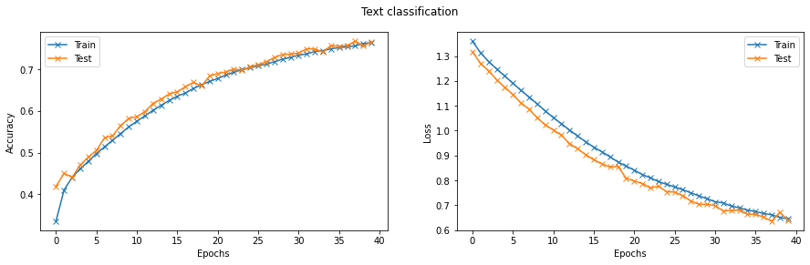
Finally, we can train and test the network. We will train the network for ten epochs. The network reached close to \(80\%\) accuracy on the test set.
# Hyperparameters
initial_epoch = 0
epochs = 40
lr = 0.1

model = TextClassificationNet(vocab_size, emb_size, num_classes).to(device)

criterion = torch.nn.CrossEntropyLoss().to(device)
optimiser = torch.optim.SGD(model.parameters(), lr=lr)

train_logs = {'acc': [], 'loss': []}
val_logs = {'acc': [], 'loss': []}
for epoch in range(initial_epoch, epochs):
    print('Epoch [%.2d]' % epoch)
    train_log = epoch_loop(model, train_loader, criterion, optimiser)

    val_log = epoch_loop(model, test_loader, criterion, None)

    print('Train     loss=%.4f     acc=%0.2f    Test     loss=%.4f     acc=%0.2f' %
          (
              np.mean(train_log[1]), np.mean(train_log[0]),
              np.mean(val_log[1]), np.mean(val_log[0])
          ))
    train_logs['acc'].append(np.mean(train_log[0]))
    train_logs['loss'].append(np.mean(train_log[1]))
    val_logs['acc'].append(np.mean(val_log[0]))
    val_logs['loss'].append(np.mean(val_log[1]))
Epoch [00]
Train     loss=1.3597     acc=0.34    Test     loss=1.3173     acc=0.42
Epoch [01]
Train     loss=1.3134     acc=0.41    Test     loss=1.2706     acc=0.45
Epoch [02]
Train     loss=1.2780     acc=0.44    Test     loss=1.2402     acc=0.44
Epoch [03]
Train     loss=1.2481     acc=0.46    Test     loss=1.2043     acc=0.47
Epoch [04]
Train     loss=1.2197     acc=0.48    Test     loss=1.1740     acc=0.49
Epoch [05]
Train     loss=1.1905     acc=0.50    Test     loss=1.1460     acc=0.51
Epoch [06]
Train     loss=1.1622     acc=0.51    Test     loss=1.1112     acc=0.54
Epoch [07]
Train     loss=1.1351     acc=0.53    Test     loss=1.0866     acc=0.54
Epoch [08]
Train     loss=1.1076     acc=0.55    Test     loss=1.0517     acc=0.57
Epoch [09]
Train     loss=1.0792     acc=0.56    Test     loss=1.0229     acc=0.58
Epoch [10]
Train     loss=1.0525     acc=0.58    Test     loss=1.0028     acc=0.59
Epoch [11]
Train     loss=1.0278     acc=0.59    Test     loss=0.9819     acc=0.60
Epoch [12]
Train     loss=1.0026     acc=0.60    Test     loss=0.9479     acc=0.62
Epoch [13]
Train     loss=0.9782     acc=0.61    Test     loss=0.9276     acc=0.63
Epoch [14]
Train     loss=0.9555     acc=0.63    Test     loss=0.9033     acc=0.64
Epoch [15]
Train     loss=0.9335     acc=0.64    Test     loss=0.8829     acc=0.65
Epoch [16]
Train     loss=0.9152     acc=0.64    Test     loss=0.8663     acc=0.66
Epoch [17]
Train     loss=0.8946     acc=0.65    Test     loss=0.8537     acc=0.67
Epoch [18]
Train     loss=0.8739     acc=0.66    Test     loss=0.8563     acc=0.66
Epoch [19]
Train     loss=0.8573     acc=0.67    Test     loss=0.8085     acc=0.68
Epoch [20]
Train     loss=0.8413     acc=0.68    Test     loss=0.7978     acc=0.69
Epoch [21]
Train     loss=0.8237     acc=0.69    Test     loss=0.7874     acc=0.69
Epoch [22]
Train     loss=0.8099     acc=0.69    Test     loss=0.7693     acc=0.70
Epoch [23]
Train     loss=0.7951     acc=0.70    Test     loss=0.7767     acc=0.70
Epoch [24]
Train     loss=0.7841     acc=0.70    Test     loss=0.7545     acc=0.71
Epoch [25]
Train     loss=0.7733     acc=0.71    Test     loss=0.7529     acc=0.71
Epoch [26]
Train     loss=0.7627     acc=0.71    Test     loss=0.7388     acc=0.72
Epoch [27]
Train     loss=0.7502     acc=0.72    Test     loss=0.7173     acc=0.73
Epoch [28]
Train     loss=0.7376     acc=0.72    Test     loss=0.7040     acc=0.74
Epoch [29]
Train     loss=0.7264     acc=0.73    Test     loss=0.7038     acc=0.74
Epoch [30]
Train     loss=0.7141     acc=0.73    Test     loss=0.6984     acc=0.74
Epoch [31]
Train     loss=0.7095     acc=0.74    Test     loss=0.6775     acc=0.75
Epoch [32]
Train     loss=0.6969     acc=0.74    Test     loss=0.6784     acc=0.75
Epoch [33]
Train     loss=0.6895     acc=0.74    Test     loss=0.6810     acc=0.74
Epoch [34]
Train     loss=0.6804     acc=0.75    Test     loss=0.6639     acc=0.76
Epoch [35]
Train     loss=0.6746     acc=0.75    Test     loss=0.6632     acc=0.76
Epoch [36]
Train     loss=0.6668     acc=0.75    Test     loss=0.6522     acc=0.76
Epoch [37]
Train     loss=0.6617     acc=0.76    Test     loss=0.6358     acc=0.77
Epoch [38]
Train     loss=0.6510     acc=0.76    Test     loss=0.6720     acc=0.76
Epoch [39]
Train     loss=0.6456     acc=0.76    Test     loss=0.6400     acc=0.77
Training progress#
Let’s plot the evolution of loss and accuracy for both train and test sets.
fig = plt.figure(figsize=(15, 4))
fig.suptitle('Text classification')
# accuraccy
ax = fig.add_subplot(1, 2, 1)
ax.plot(np.array(train_logs['acc']), '-x', label="Train")
ax.plot(np.array(val_logs['acc']), '-x', label="Test")
ax.set_xlabel("Epochs")
ax.set_ylabel("Accuracy")
ax.legend()
# loss
ax = fig.add_subplot(1, 2, 2)
ax.plot(np.array(train_logs['loss']), '-x', label="Train")
ax.plot(np.array(val_logs['loss']), '-x', label="Test")
ax.set_xlabel("Epochs")
ax.set_ylabel("Loss")
ax.legend()
plt.show()
Prediction#
Let’s try our network with some news copy-pasted from Deutsche Welle.
def predict(text):
    with torch.no_grad():
        text = torch.tensor(db_vocab(tokeniser(text)))
        output = model(text.unsqueeze(dim=0).to(device))
        return output.argmax(dim=1).item()
ex_text_str = "Magnus Carlsen is now an ex-world champion after the Norwegian, 32, \
    abdicated the crown he had held with distinction for a decade. This week and next \
    the legend takes on the pair who met for his vacated title, in a new concept for \
    chess. The Tech Mahindra Global League (GCL) has six grandmaster teams, chosen by \
    franchise auction, competing in Dubai from June 21 to July 2."

print("This is a %s news" % ag_news_labels[predict(ex_text_str)])

ex_text_str = "The worldwide spice trade has a volume of some 130 billion dollars. \
    Demand for ever more exotic spices is rising. Estimates suggest that the spice \
    industry will grow by 37 percent this year over last year. We visit a spice \
    trader in Hamburg."

print("This is a %s news" % ag_news_labels[predict(ex_text_str)])
This is a Sports news
This is a Business news
Excercises#
Below is a list of exercises to practice what we have learnt in this notebook:
Visualise or print the values of the
EmbeddingBaglayer and compute its output for a simple text sentence.
References#
The following sources inspire the materials in this notebook: