5.2. Deep Autoencoders

The materials in this notebook are inspired from:

• code

  • https://avandekleut.github.io/vae/

  • https://keras.io/examples/generative/vae/

• article https://arxiv.org/pdf/1906.02691.pdf

This tutorial covers the basics of autoencoders and Variational Autoencoders (VAE). The primary idea behind autoencoder is to learn efficient codings of unlabeled data. The architecture of a deep autoencoder consists of three components:

1. Encoder gradually reduces the dimensionality of the input \(X\) to a latent space \(Z\).

2. Latent space (also known as embedding space) is a bottleneck containing the compressed data.

3. Decoder reconstructs the signal (\(X'\)) from the latent space \(Z\).

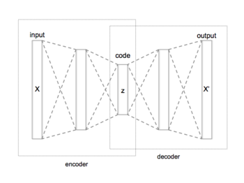
We measure the success of the network by comparing its output (\(X'\)) to input (\(X\)). The closer they are the better.

We explore a few new toy examples all in images of small resolution (\(\le32 \times 32\)):

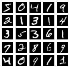
• MNIST: grey-scale digit recognition from 0 to 9.

• Fashion-MNIST grey-scale image recognition among 10 categories.

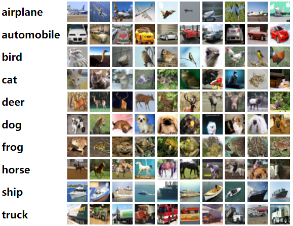
• CIFAR10: object recognition among 10 categories.

0. Packages

Let’s start with all the necessary packages to implement this tutorial.

• numpy is the main package for scientific computing with Python. It’s often imported with the np shortcut.

• argparse is a module making it easy to write user-friendly command-line interfaces.

• matplotlib is a library to plot graphs in Python.

• os provides a portable way of using operating system-dependent functionality, e.g., modifying files/folders.

• torch is a deep learning framework that allows us to define networks, handle datasets, optimise a loss function, etc.

# importing the necessary packages/libraries
import numpy as np
import argparse
from matplotlib import pyplot as plt
import random
import os
import math

import torch
import torch.nn as nn
import torchvision

device

Choosing CPU or GPU based on the availability of the hardware.

device = torch.device('cuda' if torch.cuda.is_available() else 'cpu')

arguments

We use the argparse module to define a set of parameters that we use throughout this notebook:

• The argparse is particularly useful when writing Python scripts, allowing you to run the same script with different parameters (e.g., for doing different experiments).

• In notebooks using argparse is not necessarily beneficial, we could have hard-coded those values directly in variables, but here we use argparse for learning purposes.

parser = argparse.ArgumentParser()
parser.add_argument("--n_epochs", type=int, default=20, help="number of epochs of training")
parser.add_argument("--batch_size", type=int, default=128, help="size of the batches")
parser.add_argument("--lr", type=float, default=0.0001, help="adam: learning rate")
parser.add_argument("--b1", type=float, default=0.9, help="adam: decay of first order momentum of gradient")
parser.add_argument("--b2", type=float, default=0.999, help="adam: decay of first order momentum of gradient")
parser.add_argument("--latent_dim", type=int, default=2, help="dimensionality of the latent space")
parser.add_argument("--img_size", type=int, default=32, help="size of each image dimension")
parser.add_argument("--channels", type=int, default=1, help="number of image channels")
parser.add_argument("--sample_interval", type=int, default=500, help="interval between image sampling")
parser.add_argument("--out_dir", type=str, default="./vae_out/", help="the output directory")
parser.add_argument("--dataset", type=str, default="mnist", 
                    choices=["mnist", "fashion-mnist", "cifar10"], help="which dataset to use")

def set_args(*args):
    # we can pass arguments to the parse_args function to change the default values. 
    opt = parser.parse_args([*args])
    # adding the dataset to the out dir to avoid overwriting the generated images
    opt.out_dir = "%s/%s/" % (opt.out_dir, opt.dataset)
    
    # the images in cifar10 are colourful
    if opt.dataset == "cifar10":
        opt.channels = 3
    
    # creating the output directory
    os.makedirs(opt.out_dir, exist_ok=True)
    return opt

opt = set_args("--n_epochs", "5", "--dataset", "mnist")
print(opt)

Namespace(n_epochs=5, batch_size=128, lr=0.0001, b1=0.9, b2=0.999, latent_dim=2, img_size=32, channels=1, sample_interval=500, out_dir='./vae_out//mnist/', dataset='mnist')

Architecture

class Encoder(nn.Module):
    def __init__(self, opt):
        super(Encoder, self).__init__()
        num_features = 64
        self.main = nn.Sequential(
            # input is ``(opt.channels) x opt.img_size x opt.img_size``
            nn.Conv2d(opt.channels, num_features, 4, 2, 1, bias=False),
            nn.ReLU(inplace=True),
            # state size. ``(num_features) x opt.img_size/2 x opt.img_size/2``
            nn.Conv2d(num_features, num_features * 2, 4, 2, 1, bias=False),
            nn.BatchNorm2d(num_features * 2),
            nn.ReLU(inplace=True),
            # state size. ``(num_features*2) x opt.img_size/4 x opt.img_size/4``
            nn.Conv2d(num_features * 2, num_features * 4, 4, 2, 1, bias=False),
            nn.BatchNorm2d(num_features * 4),
            nn.ReLU(inplace=True),
            # state size. ``(num_features*4) x opt.img_size/8 x opt.img_size/8``
            nn.Conv2d(num_features * 4, num_features * 8, 4, 2, 1, bias=False),
            nn.BatchNorm2d(num_features * 8),
            nn.ReLU(inplace=True),
            # state size. ``(num_features*8) x opt.img_size/16 x opt.img_size/16``
            nn.Conv2d(num_features * 8, opt.latent_dim, 2, bias=False),
        )
    
    def forward(self, x):
        x = self.main(x)
        return x

class Decoder(nn.Module):
    def __init__(self, opt):
        super(Decoder, self).__init__()
        self.out_size = (opt.img_size, opt.img_size)
        num_features = 64
        self.main = nn.Sequential(
            # input is Z, going into a convolution
            nn.ConvTranspose2d(opt.latent_dim, num_features * 8, 4, 1, 0, bias=False),
            nn.BatchNorm2d(num_features * 8),
            nn.ReLU(True),
            # state size. ``(num_features*8) x 4 x 4``
            nn.ConvTranspose2d(num_features * 8, num_features * 4, 4, 2, 1, bias=False),
            nn.BatchNorm2d(num_features * 4),
            nn.ReLU(True),
            # state size. ``(num_features*4) x 8 x 8``
            nn.ConvTranspose2d(num_features * 4, num_features * 2, 4, 2, 1, bias=False),
            nn.BatchNorm2d(num_features * 2),
            nn.ReLU(True),
            # state size. ``(num_features*2) x 16 x 16``
            nn.ConvTranspose2d(num_features * 2, num_features, 4, 2, 1, bias=False),
            nn.BatchNorm2d(num_features),
            nn.ReLU(True),
            # state size. ``(num_features) x 32 x 32``
            nn.ConvTranspose2d(num_features, opt.channels, 1, bias=False),
            # state size. ``(opt.channels) x 32 x 32``
            nn.Tanh()
        )

    def forward(self, input):
        x = self.main(input)
        return x

class Autoencoder(nn.Module):
    def __init__(self, latent_dims):
        super(Autoencoder, self).__init__()
        self.encoder = Encoder(latent_dims)
        self.decoder = Decoder(latent_dims)
    
    def forward(self, x):
        z = self.encoder(x)
        return self.decoder(z)

Next, we will write some code to train the autoencoder on the MNIST dataset.

Dataset

We explore three datasets all already implemented in torchvision. The first time will be automatically downloaded (in “./data/” directory) the first time if already it doesn’t exist.

def get_dataloader(opt, transform):
    if opt.dataset == "mnist":
        dataset = torchvision.datasets.MNIST("./data/", train=True, download=True, transform=transform)
    elif opt.dataset == "fashion-mnist":
        dataset = torchvision.datasets.FashionMNIST("./data/", train=True, download=True, transform=transform)
    else:
        dataset = torchvision.datasets.cifar.CIFAR10("./data/", train=True, download=True, transform=transform)
    return torch.utils.data.DataLoader(dataset, batch_size=opt.batch_size, shuffle=True)

Transform functions

We resize all images to specified image size (opt.img_size), converting them to Tensor and normalising the inputs (Normalize).

# make the pytorch datasets
mean = 0.5
std = 0.5
transform = torchvision.transforms.Compose([
    torchvision.transforms.Resize(opt.img_size),
    torchvision.transforms.ToTensor(),
    torchvision.transforms.Normalize(mean, std)
])

dataloader = get_dataloader(opt, transform)

Visualisation

Let’s visualise a few samples from our dataset.

fig = plt.figure(figsize=(5, 5))
for i in range(25):
    img, target = dataloader.dataset.__getitem__(i)
    ax = fig.add_subplot(5, 5, i+1)
    ax.imshow(img.numpy().transpose(1, 2, 0) * std + mean, cmap='gray')
    ax.axis('off')

Training

Setup Networks and Optimiser

def setup_training(opt, vae=False):
    # Initialise network
    network = VariationalAutoencoder(opt) if vae else Autoencoder(opt)
    network.to(device)

    # Optimiser
    optimizer = torch.optim.Adam(network.parameters(), lr=opt.lr, betas=(opt.b1, opt.b2))

    return network, optimizer

Loss

criterion = nn.MSELoss().to(device)

Utility functions

def sample_image(network, batches_done):
   with torch.no_grad():
       imgs, _ = next(iter(dataloader))
       output = network(imgs.to(device))
   torchvision.utils.save_image(
        output.data, "%s/%.7d.png" % (opt.out_dir, batches_done), nrow=10, normalize=True
    )

The training loop is straightforward:

• We input the autoencoder with input images.

• Computing the loss (MSE) of reconstructed outputs with respect to the original images.

• Optimising the network parameters.

def train_instance(opt, vae=False):
    network, optimiser = setup_training(opt, vae)

    losses = []
    for epoch in range(opt.n_epochs):
        # For each batch in the dataloader
        for i, (imgs, _) in enumerate(dataloader):
            imgs = imgs.to(device)
            optimiser.zero_grad()
            output = network(imgs)
            loss = criterion(output, imgs) + (network.encoder.kld if vae else 0)
            loss.backward()
            optimiser.step()

            losses.append(loss.item())
            
            batches_done = epoch * len(dataloader) + i
            if batches_done % opt.sample_interval == 0:
                sample_image(network, batches_done)
                print(
                    "[Epoch %.3d/%d]\t[Batch %.4d/%d]\t[loss: %.4f]"
                    % (epoch, opt.n_epochs, i, len(dataloader), np.mean(losses))
                )
    return network, losses

Results

Let’s train our autoencoder with current arguments (opt).

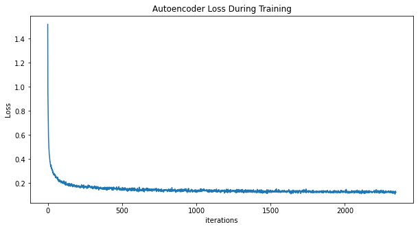
Training progress:

• loss value we can observe that the MSE (L2 norm) is gradually decreasing.

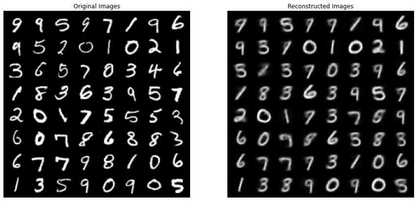
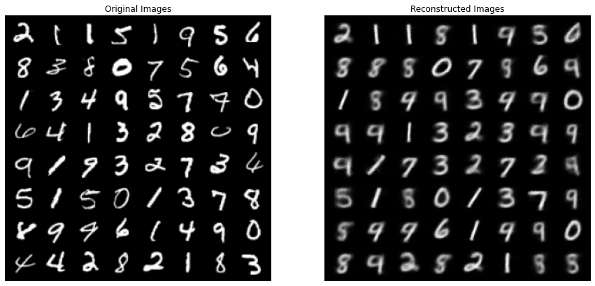
• reconstructed images By looking at the reconstructed images (in the opt.out_dir folder), we can observe that the quality of reconstructed images is quite good, given our latent space contains only 2 units. In other words, each image is compressed into only two numbers.

autoencoder, losses = train_instance(opt)

[Epoch 000/5]	[Batch 0000/469]	[loss: 1.5200]
[Epoch 001/5]	[Batch 0031/469]	[loss: 0.1983]
[Epoch 002/5]	[Batch 0062/469]	[loss: 0.1709]
[Epoch 003/5]	[Batch 0093/469]	[loss: 0.1590]
[Epoch 004/5]	[Batch 0124/469]	[loss: 0.1519]

plt.figure(figsize=(10,5))
plt.title("Autoencoder Loss During Training")
plt.plot(losses)
plt.xlabel("iterations")
plt.ylabel("Loss")
plt.show()

Reconstructing

# Grab a batch of real images from the dataloader
org_batch = next(iter(dataloader))

# Plot the real images
plt.figure(figsize=(15,15))
plt.subplot(1,2,1)
plt.axis("off")
plt.title("Original Images")
plt.imshow(np.transpose(torchvision.utils.make_grid(org_batch[0][:64], padding=5, normalize=True).cpu(),(1,2,0)))


with torch.no_grad():
    reconstructed_imgs = autoencoder(org_batch[0].to(device)).detach().cpu()

# Plot the fake images from the last epoch
plt.subplot(1,2,2)
plt.axis("off")
plt.title("Reconstructed Images")
plt.imshow(np.transpose(torchvision.utils.make_grid(reconstructed_imgs[:64], padding=5, normalize=True).cpu(),(1,2,0)))
plt.show()

Latent space

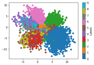
One interesting aspect of autoencoders is that we can explore the latent space to learn more about the structure of representation in a network.

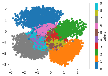
We create the plot_latent function which visualises both dimensions of our latent space, colour-coding each point according to the label of the image. In this function, we only call the encoder part of our model.

Note This simple visualisation only works if the dimensionality of the latent space is two. For hyperdimensional latent spaces, you can use sklearn.manifold.TSNE to reduce the dimensionality to 2.

def plot_latent(autoencoder, dataloader, num_batches=100):
    for i, (imgs, labels) in enumerate(dataloader):
        # only calling the encoder part of our network
        z = autoencoder.encoder(imgs.to(device))
        z = z.to('cpu').detach().numpy()
        plt.scatter(z[:, 0], z[:, 1], c=labels, cmap='tab10')
        if i > num_batches:
            cbar = plt.colorbar()
            cbar.set_label('Labels')
            break

We can notice that:

• The latent space of our network has some meaningful structure.

• The range of the x- and y-axis is not the same and the data points are elongated.

• Although categories are relatively separated, there is also some significant degree of overlapping.

plot_latent(autoencoder, dataloader)

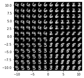
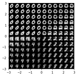
We use the range of values in the x- and y-axis to generate new samples directly from the latent space.

We create a function plot_reconstructed that only calls de decoder part of our model to uniformly sample from the latent space.

Note This simple visualisation only works if the dimensionality of the latent space is two. For hyperdimensional latent spaces, you can use sklearn.manifold.TSNE to reduce the dimensionality to 2.

def plot_reconstructed(autoencoder, opt, r0, r1, n=12):
    w = opt.img_size
    img = np.zeros((n*w, n*w, opt.channels)).squeeze()
    for i, y in enumerate(np.linspace(*r1, n)):
        for j, x in enumerate(np.linspace(*r0, n)):
            z = torch.Tensor([[x, y]]).unsqueeze(dim=-1).unsqueeze(dim=-1).to(device)
            x_hat = autoencoder.decoder(z)
            x_hat = x_hat.to('cpu').detach().numpy().squeeze() * std + mean
            if opt.channels == 3:
                x_hat = x_hat.transpose(1, 2, 0)
            img[(n-1-i)*w:(n-1-i+1)*w, j*w:(j+1)*w] = x_hat
    plt.imshow(img, extent=[*r0, *r1], cmap='gray')

plot_reconstructed(autoencoder, opt, (-11, 11), (-11, 11))

Variational Autoencoder (VAE)

The latent space (\(Z\)) of our autoencoder doesn’t have any constraint. In VAEs, the encoder maps the input into probability distributions. The decoder receives a sample from these distributions. Specifically, the encoder maps the input into two vectors:

• mean vector \(\mu(x)\)

• standard deviation \(\sigma(x)\)

The output of encoder is reparameterised into \(z\) and passed to the decoder. Read more about it in Wikipedia.

Architecture

We implement this in VariationalEncoder:

• The sequence of layers in VariationalEncoder.main is identical to Encoder except the last layer.

• Instead of one nn.Conv2d(num_features * 8, opt.latent_dim, 2) we have two corresponding to \(\mu\) and \(\sigma\).

• The forward function is quite different. It calls the reparameterise function to sample \(z\).

Note: we have not changed the Decoder.

class VariationalEncoder(nn.Module):
    def __init__(self, opt):
        super(VariationalEncoder, self).__init__()
        num_features = 64
        self.main = nn.Sequential(
            # input is ``(opt.channels) x opt.img_size x opt.img_size``
            nn.Conv2d(opt.channels, num_features, 4, 2, 1, bias=False),
            nn.ReLU(inplace=True),
            # state size. ``(num_features) x opt.img_size/2 x opt.img_size/2``
            nn.Conv2d(num_features, num_features * 2, 4, 2, 1, bias=False),
            nn.BatchNorm2d(num_features * 2),
            nn.ReLU(inplace=True),
            # state size. ``(num_features*2) x opt.img_size/4 x opt.img_size/4``
            nn.Conv2d(num_features * 2, num_features * 4, 4, 2, 1, bias=False),
            nn.BatchNorm2d(num_features * 4),
            nn.ReLU(inplace=True),
            # state size. ``(num_features*4) x opt.img_size/8 x opt.img_size/8``
            nn.Conv2d(num_features * 4, num_features * 8, 4, 2, 1, bias=False),
            nn.BatchNorm2d(num_features * 8),
            nn.ReLU(inplace=True),
        )

        # state size. ``(num_features*8) x opt.img_size/16 x opt.img_size/16``
        self.mu_layer = nn.Conv2d(num_features * 8, opt.latent_dim, 2)
        self.sigma_layer = nn.Conv2d(num_features * 8, opt.latent_dim, 2)

        # Kullback–Leibler divergence
        self.kld = 0
        self.kld_weight = 1e-3

    def reparameterise(self, mu, sigma):
        return mu + sigma * torch.randn_like(mu)

    def set_kld_loss(self, mu, sigma):
        self.kld = sigma.pow(2) + mu.pow(2) - torch.log(sigma) - 0.5
        self.kld = torch.mean(torch.sum(self.kld, dim=1))
        self.kld *= self.kld_weight
        
    def forward(self, x):
        x = self.main(x)
        mu = self.mu_layer(x)
        sigma = torch.exp(self.sigma_layer(x))
        z = self.reparameterise(mu, sigma)
        self.set_kld_loss(mu, sigma)
        return z

class VariationalAutoencoder(nn.Module):
    def __init__(self, latent_dims):
        super(VariationalAutoencoder, self).__init__()
        self.encoder = VariationalEncoder(latent_dims)
        self.decoder = Decoder(latent_dims)
    
    def forward(self, x):
        z = self.encoder(x)
        return self.decoder(z)

Loss

In VAE, we add the Kullback-Leibler divergence loss to the MSE loss. We have implemented this in VariationalEncoder in the kld variable. Therefore, in the train_instance function, the loss is computed as:

loss = criterion(output, imgs) + (network.encoder.kld if vae else 0)

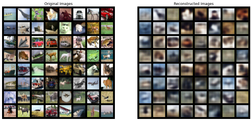
Results

Let’s train a VAE with current arguments (opt).

vae_net, losses = train_instance(opt, vae=True)

[Epoch 000/5]	[Batch 0000/469]	[loss: 2.1240]
[Epoch 001/5]	[Batch 0031/469]	[loss: 0.2317]
[Epoch 002/5]	[Batch 0062/469]	[loss: 0.1957]
[Epoch 003/5]	[Batch 0093/469]	[loss: 0.1802]
[Epoch 004/5]	[Batch 0124/469]	[loss: 0.1711]

Reconstructing

# Grab a batch of real images from the dataloader
org_batch = next(iter(dataloader))

# Plot the real images
plt.figure(figsize=(15,15))
plt.subplot(1,2,1)
plt.axis("off")
plt.title("Original Images")
plt.imshow(np.transpose(torchvision.utils.make_grid(org_batch[0][:64], padding=5, normalize=True).cpu(),(1,2,0)))


with torch.no_grad():
    reconstructed_imgs = vae_net(org_batch[0].to(device)).detach().cpu()

# Plot the fake images from the last epoch
plt.subplot(1,2,2)
plt.axis("off")
plt.title("Reconstructed Images")
plt.imshow(np.transpose(torchvision.utils.make_grid(reconstructed_imgs[:64], padding=5, normalize=True).cpu(),(1,2,0)))
plt.show()

Latent space

Similar to the autoencoder we can inspect the VAE’s latent space. We observe that:

• The distribution of data points resembles a Gaussian distribution (more centralised).

• The range of x- and y-axis are more bound.

plot_latent(vae_net, dataloader)

plot_reconstructed(vae_net, opt, (-3, 3), (-3, 3))

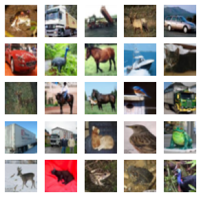
Another dataset

Let’s play with another dataset!

opt = set_args("--n_epochs", "5", "--dataset", "cifar10", "--latent_dim", "100")
print(opt)

dataloader = get_dataloader(opt, transform)

fig = plt.figure(figsize=(5, 5))
for i in range(25):
    img, target = dataloader.dataset.__getitem__(i)
    ax = fig.add_subplot(5, 5, i+1)
    ax.imshow(img.numpy().transpose(1, 2, 0) * std + mean, cmap='gray')
    ax.axis('off')

Namespace(n_epochs=5, batch_size=128, lr=0.0001, b1=0.9, b2=0.999, latent_dim=100, img_size=32, channels=3, sample_interval=500, out_dir='./vae_out//cifar10/', dataset='cifar10')
Files already downloaded and verified

vae_net, losses = train_instance(opt, vae=True)

[Epoch 000/5]	[Batch 0000/391]	[loss: 0.9570]
[Epoch 001/5]	[Batch 0109/391]	[loss: 0.2267]
[Epoch 002/5]	[Batch 0218/391]	[loss: 0.2030]
[Epoch 003/5]	[Batch 0327/391]	[loss: 0.1884]

# Grab a batch of real images from the dataloader
org_batch = next(iter(dataloader))

# Plot the real images
plt.figure(figsize=(15,15))
plt.subplot(1,2,1)
plt.axis("off")
plt.title("Original Images")
plt.imshow(np.transpose(torchvision.utils.make_grid(org_batch[0][:64], padding=5, normalize=True).cpu(),(1,2,0)))


with torch.no_grad():
    reconstructed_imgs = vae_net(org_batch[0].to(device)).detach().cpu()

# Plot the fake images from the last epoch
plt.subplot(1,2,2)
plt.axis("off")
plt.title("Reconstructed Images")
plt.imshow(np.transpose(torchvision.utils.make_grid(reconstructed_imgs[:64], padding=5, normalize=True).cpu(),(1,2,0)))
plt.show()