6.1. Activation Maps

This tutorial showcases how to obtain kernels’ responses (also known as activation maps) at different depths of a deep neural network. We study that in pretrained networks trained on ImageNet.

In neuroscience, we have learnt a lot from measuring the response of a neuron when the organism is exposed to specific stimuli. The neural coding technique can reveal the relationship between the stimulus and the individual or ensemble neuronal responses. For instance, the seminal study of Hubel and Wiesel in which oriented bars were shown to cats and the response of V1 neurons was recorded using implanted electrodes.

A similar technique can be used in artificial neurons to learn more about the representation a network has learnt during its training. Obtaining response maps is much easier in deep networks:

• we can show them numerous stimuli,

• we have access to all units.

Example articles that use this technique:

• Contrast sensitivity functions in autoencoders

• Color for object recognition: Hue and chroma sensitivity in the deep features of convolutional neural networks

0. Packages

Let’s start with all the necessary packages to implement this tutorial.

• numpy is the main package for scientific computing with Python. It’s often imported with the np shortcut.

• matplotlib is a library to plot graphs in Python.

• os provides a portable way of using operating system-dependent functionality, e.g., modifying files/folders.

• requests is a package that collects several modules for working with URLs.

• PIL is a fast image processing designed for general applications.

• torch is a deep learning framework that allows us to define networks, handle datasets, optimise a loss function, etc.

# importing the necessary packages/libraries
import numpy as np
from matplotlib import pyplot as plt
import random
import os
import requests

from PIL import Image as pil_image

import torch
import torchvision
from torchvision import models
import torchvision.transforms as torch_transforms

device

Choosing CPU or GPU based on the availability of the hardware.

device = torch.device('cuda' if torch.cuda.is_available() else 'cpu')

1. Stimuli

In this tutorial, we use natural images as our stimuli, but one can show artificial networks any type of stimuli.

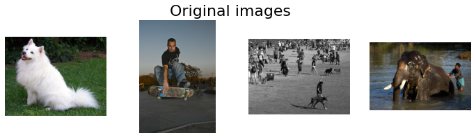
We load four images from the internet and show them.

# list of image URLs
urls = [
    'https://github.com/pytorch/hub/raw/master/images/dog.jpg',
    'http://farm4.staticflickr.com/3418/3368475823_74f3d3e9f9_z.jpg', 
    'http://farm3.staticflickr.com/2431/3908162999_5b5cd7c1b7_z.jpg',
    'http://farm8.staticflickr.com/7069/6903096875_042efb5ee7_z.jpg'
]

# Openning the image and visualising it
input_images = [pil_image.open(requests.get(url, stream=True).raw) for url in urls]

fig = plt.figure(figsize=(12, 3))
fig.suptitle('Original images', size=22)
for img_ind, img in enumerate(input_images):
    ax = fig.add_subplot(1, 4, img_ind+1)
    ax.imshow(img)
    ax.axis('off')

Torch Tensors

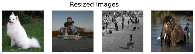
Before inputting a network with our images we:

1. resize them to what the image size that the pretrained network was trained on,

2. normalise them to the range of values that the pretrained network was trained on.

While these two steps are not strictly speaking mandatory, it’s sensible to measure the response of kernels under similar conditions that the network is meant to function.

In the end, we visualise the tensor images (after inverting the normalisation). This is often a good exercise to do to ensure what we show to networks is correct.

# the training size of ImageNet pretrained networks
target_size = 224
# mean and std values of ImageNet pretrained networks
mean = [0.485, 0.456, 0.406]
std = [0.229, 0.224, 0.225]

# the list of transformation functions
transforsm = torch_transforms.Compose([
    torch_transforms.Resize((target_size, target_size)),
    torch_transforms.ToTensor(),
    torch_transforms.Normalize(mean=mean, std=std)
])

torch_imgs = torch.stack([transforsm(img) for img in input_images])
print("Input tensor shape:", torch_imgs.shape)

# visualising the torch images
fig = plt.figure(figsize=(12, 3))
fig.suptitle('Resized images', size=22)
for img_ind, img in enumerate(torch_imgs):
    ax = fig.add_subplot(1, 4, img_ind+1)
    # inversing the normalisation by multiplying to std and adding mean
    ax.imshow(img.numpy().transpose(1, 2, 0) * std + mean)
    ax.axis('off')

Clipping input data to the valid range for imshow with RGB data ([0..1] for floats or [0..255] for integers).
Clipping input data to the valid range for imshow with RGB data ([0..1] for floats or [0..255] for integers).

Input tensor shape: torch.Size([4, 3, 224, 224])

2. Network

We use torchvision.models to obtain networks pretrained on ImageNet.

In this tutorial, we focus on the ResNet architectures, but the logic of computing activation maps remains the same for all other convolutional neural networks (CNN).

Remember that you must call network.eval() to set dropout and batch normalisation layers to evaluation mode before recording activation maps. Failing to do this will yield inconsistent results.

network = models.resnet50(weights=models.ResNet50_Weights.IMAGENET1K_V1).to(device)
network.eval()

# getting the name of layers, which we use later to obtain their activation maps
layer_names = [key for key, _ in network.named_children()]
print(layer_names)

['conv1', 'bn1', 'relu', 'maxpool', 'layer1', 'layer2', 'layer3', 'layer4', 'avgpool', 'fc']

3. Forward Hooks

PyTorch allows inspecting/modifying the output and gradient output of a layer using hooks. In this tutorial, we use forward hooks to inspect the output of a layer. To do so, we call the register_forward_hook for every layer that we want to inspect:

• register_forward_hook registers a forward hook on the module.

• The hook will be called every time after forward() has computed an output.

• It returns a handle that can be used to remove the added hook by calling handle.remove().

The hook should have the following signature:

hook(module, args, output) -> None or modified output

In our example, we have implemented this in the activation function that stores the outputs in a dict.

In our example, we only access the first tier of layers/modules that are accessible by

layer = getattr(model, layer_name)

Essentially, we can only access one of these ten layers:

['conv1', 'bn1', 'relu', 'maxpool', 'layer1', 'layer2', 'layer3', 'layer4', 'avgpool', 'fc']

However, many times a network consists of several nested modules. Often, we also want to record the activation maps of those layer. For instance, layer1-4 of ResNet contains several residual blocks. To access those nested layers:

• Access the parent module, for example, by calling the getattr module or simply by getting the correct index from the list of network.children().

• Iterate this process until the layer is directly accessible and it’s not nested within another module.

Excercie: create hooks for residual blocks of ResNet or hidden layers of any other network you’re interested to explore.

def activation(name, acts_dict):
    """Storing the output of a module/layer in the dict that is passed as an argument."""
    def hook(model, input_x, output_y):
        acts_dict[name] = output_y.detach()
    return hook

def create_hooks(model, layers):
    """For the given model it creates a hook for all specified layers."""
    acts_dict = dict()
    hooks = dict()
    for layer_name in layers:
        # accessing the layer/module from the network
        layer = getattr(model, layer_name)
        hooks[layer_name] = layer.register_forward_hook(activation(layer_name, acts_dict))
    return acts_dict, hooks

Next we create the hooks for three layers ['maxpool', 'layer2', 'fc'] of our network. The activation maps are filled in when we call the forward function of the networks

acts_dict, hooks = create_hooks(network, ['maxpool', 'layer2', 'fc'])

4. Forward call

Next, we simply input the network with our input stimuli torch_imgs. Note: we’re not really interested in the output of the network per see, but rather the activation maps that are filled in the acts_dict after the forward call.

Important If you call the network once again with a new set of stimuli, the data in acts_dict gets overwritten. Therefore, if you need that information you have to make a copy of then in another variable.

_ = network(torch_imgs.to(device))

5. Visualisation

Let’s look at the obtained activation maps. First, we just print the shape of obtained activation maps:

• The first dimension for all examined layers is 4 corresponding to the number of images.

• The second dimension corresponds to the number of kernels (e.g., maxpool has 64 kernels).

• The third and fourth are the spatial resolution (note that the fc layer doesn’t have any spatial content).

for layer_name, layer_acts in acts_dict.items():
    print(layer_name, layer_acts.shape)

maxpool torch.Size([4, 64, 56, 56])
layer2 torch.Size([4, 512, 28, 28])
fc torch.Size([4, 1000])

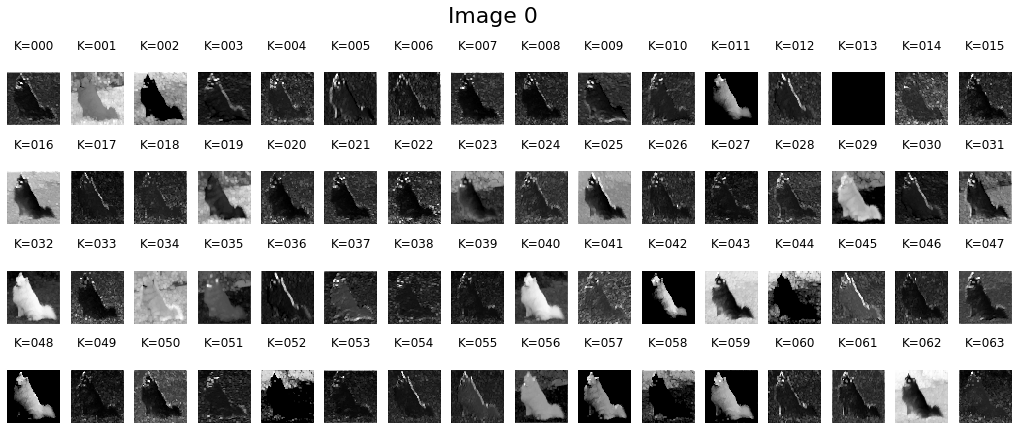
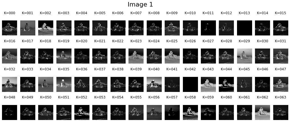
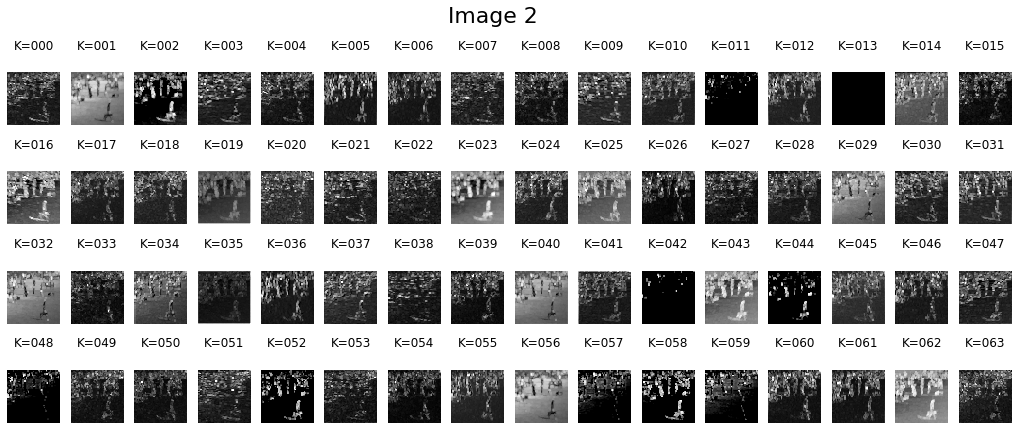
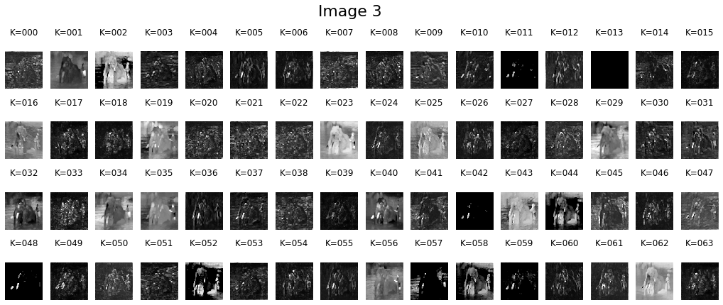
Early layer

Next, we visualise the activation maps of the maxpool layer to have some intuitions about the obtained responses. We can observe excitation by low-level features such as:

• Some of the kernels get activated by certain colours.

• Other kernels get activated by edges.

The maxpool corresponds to an early layer of ResNet50, therefore the features that kernels are responsive to are also basic features.

layer_act = acts_dict['maxpool']
for img_ind, layer_acts in enumerate(layer_act):
    fig = plt.figure(figsize=(18, 7))
    fig.suptitle('Image %d' % img_ind, size=22)
    cols = 16
    rows = layer_acts.shape[0] // cols
    for kernel_ind, kernel_act in enumerate(layer_acts.detach().cpu()):
        ax = fig.add_subplot(rows, cols, kernel_ind+1)
        ax.matshow(kernel_act, cmap='gray')
        ax.set_title('K=%.3d' % kernel_ind)
        ax.axis('off')

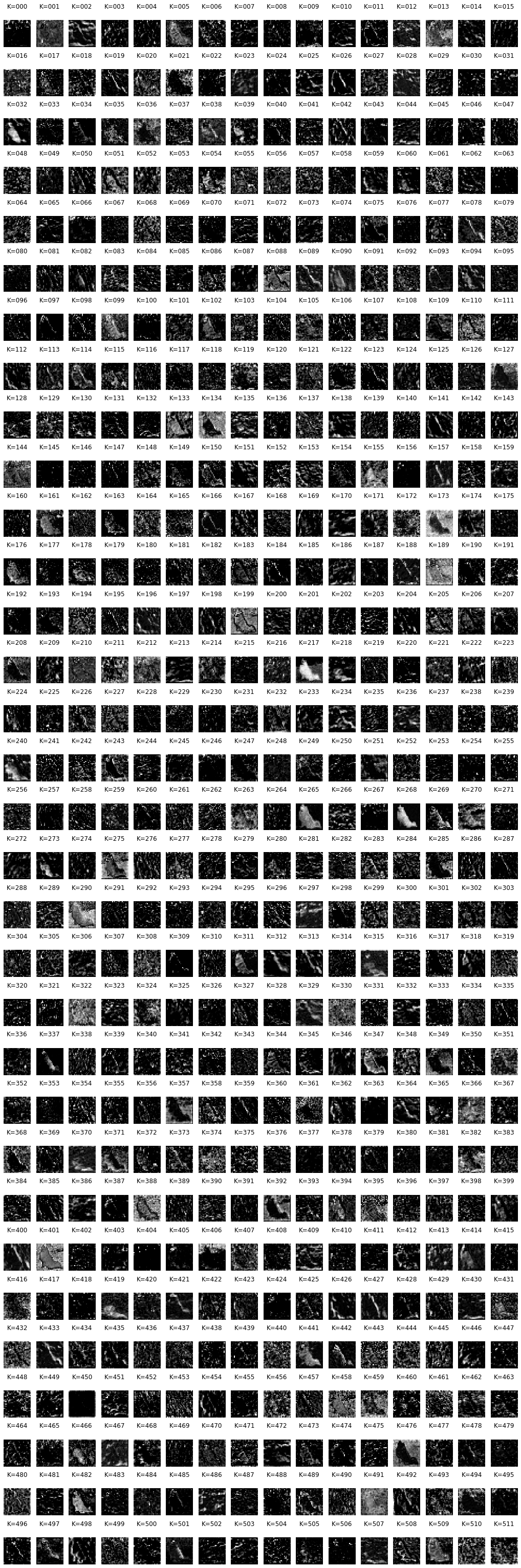
Deeper layer

Let’s visualise the activation maps of a deeper layer layer2 for one of the images. Overall, we can observe that the activation maps are not as simple as an earlier layer. Kernels in layer2 respond to different patterns and textures. The set of features that excite a kernel becomes more complex as we go deeper into a network.

layer_act = acts_dict['layer2']
for img_ind, layer_acts in enumerate(layer_act):
    fig = plt.figure(figsize=(18, 56))
    cols = 16
    rows = layer_acts.shape[0] // cols
    for kernel_ind, kernel_act in enumerate(layer_acts.detach().cpu()):
        ax = fig.add_subplot(rows, cols, kernel_ind+1)
        ax.matshow(kernel_act, cmap='gray')
        ax.set_title('K=%.3d' % kernel_ind)
        ax.axis('off')
    break

6. Systematic experiments

While visualisation of activation maps for natural images is interesting and results in some intuition about the underlying representation of deep networks, it’s more informative to check the activation maps with respect to a specific feature (i.e., dependent variable) and keep all other parameters fixed (i.e., independent variables).

Quantitative assessment: the activation maps we visualised above contain spatial resolution. To report the degree of excitation one could use different techniques such as:

• Statistics of the entire activation map (e.g., mean or median).

• Statistics on pixels corresponding to the foreground stimuli. This is only possible if we have a segmentation map of input pixels (e.g., in the case of generated stimuli).

• Thresholding the activation maps and counting the number of pixels that meet this criterion.

Questions to explore: recording the activation map is a powerful technique and one can perform many interesting experiments with it. Below are a few example exercises:

1. Colour

   • Plot a circle in the middle of a grey background.

   • Change the colour of the circle systematically across the hue spectrum.

   • Measure the activation of kernels.

   • Are there kernels that get highly excited in the presence of certain colours?

   • Are colour kernels more present in early or deeper layers?

2. Size

   • Plot different geometrical shapes in the middle of a grey background.

   • Change the size of those shapes systematically.

   • Measure the activation of kernels.

   • Plot the level of activation as a function of stimuli size.

   • Do artificial kernels show a preference for a certain size?

   • Does The size preference of kernels change as a function of layer?