6.1. Generative Adversarial Network#
The materials in this notebook are inspired from:
code
article https://arxiv.org/abs/1610.09585
This tutorial covers the basics of Generative Adversarial Networks (GAN). In a GAN, two neural networks contest with each other in the form of a zero-sum game, where one agent’s gain is another agent’s loss:
Generator is trained to create samples that fool the discriminator network.
Discriminator is trained to distinguish authentic from fake samples.

As the generator becomes better at faking samples, the discriminator becomes better at distinguishing authentic samples.
We explore a few new toy examples all in images of small resolution (\(\le32 \times 32\)):
MNIST: grey-scale digit recognition from 0 to 9.

Fashion-MNIST grey-scale image recognition among 10 categories.
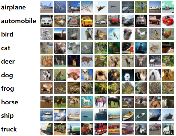
CIFAR10: object recognition among 10 categories.
0. Packages#
Let’s start with all the necessary packages to implement this tutorial.
numpy is the main package for scientific computing with Python. It’s often imported with the
npshortcut.argparse is a module making it easy to write user-friendly command-line interfaces.
matplotlib is a library to plot graphs in Python.
os provides a portable way of using operating system-dependent functionality, e.g., modifying files/folders.
torch is a deep learning framework that allows us to define networks, handle datasets, optimise a loss function, etc.
# importing the necessary packages/libraries
import numpy as np
import argparse
from matplotlib import pyplot as plt
import random
import os
import math

import torch
import torch.nn as nn
import torchvision
device#
Choosing CPU or GPU based on the availability of the hardware.
device = torch.device('cuda' if torch.cuda.is_available() else 'cpu')
arguments#
We use the argparse module to define a set of parameters that we use throughout this notebook:
The
argparseis particularly useful when writing Python scripts, allowing you to run the same script with different parameters (e.g., for doing different experiments).In notebooks using
argparseis not necessarily beneficial, we could have hard-coded those values directly in variables, but here we useargparsefor learning purposes.
parser = argparse.ArgumentParser()
parser.add_argument("--n_epochs", type=int, default=20, help="number of epochs of training")
parser.add_argument("--batch_size", type=int, default=128, help="size of the batches")
parser.add_argument("--lr", type=float, default=0.0002, help="adam: learning rate")
parser.add_argument("--b1", type=float, default=0.5, help="adam: decay of first order momentum of gradient")
parser.add_argument("--b2", type=float, default=0.999, help="adam: decay of first order momentum of gradient")
parser.add_argument("--latent_dim", type=int, default=100, help="dimensionality of the latent space")
parser.add_argument("--img_size", type=int, default=32, help="size of each image dimension")
parser.add_argument("--channels", type=int, default=1, help="number of image channels")
parser.add_argument("--sample_interval", type=int, default=500, help="interval between image sampling")
parser.add_argument("--out_dir", type=str, default="./gan_out/", help="the output directory")
parser.add_argument("--dataset", type=str, default="mnist",
                    choices=["mnist", "fashion-mnist", "cifar10"], help="which dataset to use")

def set_args(*args):
    # we can pass arguments to the parse_args function to change the default values.
    opt = parser.parse_args([*args])
    # adding the dataset to the out dir to avoid overwriting the generated images
    opt.out_dir = "%s/%s/" % (opt.out_dir, opt.dataset)

    # the images in cifar10 are colourful
    if opt.dataset == "cifar10":
        opt.channels = 3

    # creating the output directory
    os.makedirs(opt.out_dir, exist_ok=True)
    return opt
opt = set_args("--n_epochs", "5", "--dataset", "cifar10")
print(opt)
Namespace(n_epochs=5, batch_size=128, lr=0.0002, b1=0.5, b2=0.999, n_cpu=8, latent_dim=100, img_size=32, channels=3, sample_interval=500, out_dir='./gan_out//cifar10/', dataset='cifar10')
Architectures#
We have to define two architectures.
The generator is input with a noise vector (e.g., with \(100\) elements) and produces an image of size \(32 \times 32\) (either in grey-scale or colourful).
The discriminator is input with an image of \(32 \times 32\) (either in grey-scale or colourful) and determines whether the image is authentic or fake (i.e., a binary classification).
Generator#
In our implementation of the Generator we use blocks of:
Transposed convolution (
ConvTranspose2d) gradually increases the spatial resolution,Batch normalisation
BatchNorm2d,And
ReLUactivation function.
We use the Tanh to clip the outputs in the range \([-1, 1]\):

class Generator(nn.Module):
    def __init__(self, opt):
        super(Generator, self).__init__()
        self.out_size = (opt.img_size, opt.img_size)
        num_features = 64
        self.main = nn.Sequential(
            # input is Z, going into a convolution
            nn.ConvTranspose2d(opt.latent_dim, num_features * 8, 4, 1, 0, bias=False),
            nn.BatchNorm2d(num_features * 8),
            nn.ReLU(True),
            # state size. ``(num_features*8) x 4 x 4``
            nn.ConvTranspose2d(num_features * 8, num_features * 4, 4, 2, 1, bias=False),
            nn.BatchNorm2d(num_features * 4),
            nn.ReLU(True),
            # state size. ``(num_features*4) x 8 x 8``
            nn.ConvTranspose2d(num_features * 4, num_features * 2, 4, 2, 1, bias=False),
            nn.BatchNorm2d(num_features * 2),
            nn.ReLU(True),
            # state size. ``(num_features*2) x 16 x 16``
            nn.ConvTranspose2d(num_features * 2, num_features, 4, 2, 1, bias=False),
            nn.BatchNorm2d(num_features),
            nn.ReLU(True),
            # state size. ``(num_features) x 32 x 32``
            nn.ConvTranspose2d(num_features, opt.channels, 1, bias=False),
            # state size. ``(opt.channels) x 32 x 32``
            nn.Tanh()
        )

    def forward(self, input):
        return self.main(input)
Discriminator#
The Discriminator has a symmetrical architecture to the Generator using blocks of:
Convolution (
Conv2d) that gradually decreases the spatial resolution,Batch normalisation
BatchNorm2d,And
LeakyReLUactivation function.

The output is a binary classification (i.e., authentic versus fake). We use a fully convolutional implementation (i.e., the classification layer is also Conv2d instead of Linearlayer) followed by the Sigmoidactivation function.
class Discriminator(nn.Module):
    def __init__(self, opt):
        super(Discriminator, self).__init__()
        num_features = 64
        self.main = nn.Sequential(
            # input is ``(opt.channels) x opt.img_size x opt.img_size``
            nn.Conv2d(opt.channels, num_features, 4, 2, 1, bias=False),
            nn.LeakyReLU(0.2, inplace=True),
            # state size. ``(num_features) x opt.img_size/2 x opt.img_size/2``
            nn.Conv2d(num_features, num_features * 2, 4, 2, 1, bias=False),
            nn.BatchNorm2d(num_features * 2),
            nn.LeakyReLU(0.2, inplace=True),
            # state size. ``(num_features*2) x opt.img_size/4 x opt.img_size/4``
            nn.Conv2d(num_features * 2, num_features * 4, 4, 2, 1, bias=False),
            nn.BatchNorm2d(num_features * 4),
            nn.LeakyReLU(0.2, inplace=True),
            # state size. ``(num_features*4) x opt.img_size/8 x opt.img_size/8``
            nn.Conv2d(num_features * 4, num_features * 8, 4, 2, 1, bias=False),
            nn.BatchNorm2d(num_features * 8),
            nn.LeakyReLU(0.2, inplace=True),
            # state size. ``(num_features*8) x opt.img_size/16 x opt.img_size/16``
            nn.Conv2d(num_features * 8, 1, 2, bias=False),
            nn.Sigmoid()
        )

    def forward(self, input):
        return self.main(input)
Weights initialisation#
It’s a common practice to initialise the weights of GANs’ networks from a normal distribution. This has been reported experimentally to produce betetr results.
def weights_init_normal(m):
    """reinitialising all (transpose-)convolutional and batch normalization layers."""
    classname = m.__class__.__name__
    if classname.find("Conv") != -1:
        torch.nn.init.normal_(m.weight.data, 0.0, 0.02)
    elif classname.find("BatchNorm2d") != -1:
        torch.nn.init.normal_(m.weight.data, 1.0, 0.02)
        torch.nn.init.constant_(m.bias.data, 0.0)
Dataset#
We explore three datasets all already implemented in torchvision. The first time will be automatically downloaded (in “./data/” directory) the first time if already it doesn’t exist.
def get_dataloader(opt, transform):
    if opt.dataset == "mnist":
        dataset = torchvision.datasets.MNIST("./data/", train=True, download=True, transform=transform)
    elif opt.dataset == "fashion-mnist":
        dataset = torchvision.datasets.FashionMNIST("./data/", train=True, download=True, transform=transform)
    else:
        dataset = torchvision.datasets.cifar.CIFAR10("./data/", train=True, download=True, transform=transform)
    return torch.utils.data.DataLoader(dataset, batch_size=opt.batch_size, shuffle=True)
Transform functions#
We resize all images to specified image size (opt.img_size), converting them to Tensor and normalising the inputs (Normalize).
# make the pytorch datasets
mean = 0.5
std = 0.5
transform = torchvision.transforms.Compose([
    torchvision.transforms.Resize(opt.img_size),
    torchvision.transforms.ToTensor(),
    torchvision.transforms.Normalize(mean, std)
])

dataloader = get_dataloader(opt, transform)
Files already downloaded and verified
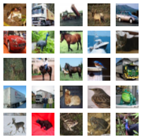
Visualisation#
Let’s visualise a few samples from our dataset.
fig = plt.figure(figsize=(5, 5))
for i in range(25):
    img, target = dataloader.dataset.__getitem__(i)
    ax = fig.add_subplot(5, 5, i+1)
    ax.imshow(img.numpy().transpose(1, 2, 0) * std + mean, cmap='gray')
    ax.axis('off')
Training#
Setup Networks and Optimiser#
def setup_training(opt):
    # Initialise generator and discriminator
    generator = Generator(opt).to(device)
    discriminator = Discriminator(opt).to(device)

    # Initialize weights
    generator.apply(weights_init_normal)
    discriminator.apply(weights_init_normal)

    # Optimisers
    optimizer_g = torch.optim.Adam(generator.parameters(), lr=opt.lr, betas=(opt.b1, opt.b2))
    optimizer_d = torch.optim.Adam(discriminator.parameters(), lr=opt.lr, betas=(opt.b1, opt.b2))

    return generator, discriminator, optimizer_g, optimizer_d
Loss and ground-truths#
# Loss functions
adversarial_loss = torch.nn.BCELoss().to(device)

# Create batch of latent vectors that we will use to visualize
#  the progression of the generator
fixed_noise = torch.randn(10 ** 2, opt.latent_dim, 1, 1, device=device)

# Establish convention for real and fake labels during training
real_label = 1.
fake_label = 0.
Utility functions#
def sample_image(generator, batches_done):
    """Saves a grid of generated images."""
    with torch.no_grad():
        gen_imgs = generator(fixed_noise).detach().cpu()
    torchvision.utils.save_image(
        gen_imgs.data, "%s/%.7d.png" % (opt.out_dir, batches_done), nrow=10, normalize=True
    )
The training loop consists of three steps:
Discriminator
First, we train the discriminator with “real” images from our dataset.
Second, we train the discriminator with “fake” images obtained from generator.
Generator
Third, we train the generator in an effort to generate better fakes.
Note: in all three steps, we use a single loss function adversarial_loss, which we defined earlier as a Binary Cross Entropy (BCELoss). In other words, we always optimise with respect to how good/bad the discriminator is in detecting real/fake images.
def train_instance(opt):
    generator, discriminator, optimizer_g, optimizer_d = setup_training(opt)

    print(generator)
    print(discriminator)

    d_losses = []
    g_losses = []
    accs_d_x = []
    accs_d_z = []

    for epoch in range(opt.n_epochs):
        # For each batch in the dataloader
        for i, (imgs, _) in enumerate(dataloader):
            imgs = imgs.to(device)
            b_size = imgs.size(0)

            # ---------------------
            #  Train Discriminator
            # ---------------------

            ## Train with all-real batch
            discriminator.zero_grad()
            label = torch.full((b_size,), real_label, dtype=torch.float, device=device)
            # Forward pass real batch through D
            output = discriminator(imgs).view(-1)
            # Calculate loss on all-real batch
            err_d_real = adversarial_loss(output, label)
            # Calculate gradients for D in backward pass
            err_d_real.backward()
            d_x = (output > 0.5).float().mean().item()

            ## Train with all-fake batch
            # Generate batch of latent vectors
            noise = torch.randn(b_size, opt.latent_dim, 1, 1, device=device)
            # Generate fake image batch with G
            fake = generator(noise)
            label.fill_(fake_label)
            # Classify all fake batch with D
            output = discriminator(fake.detach()).view(-1)
            # Calculate D's loss on the all-fake batch
            err_d_fake = adversarial_loss(output, label)
            # Calculate the gradients for this batch, accumulated (summed) with previous gradients
            err_d_fake.backward()
            d_z1 = (output < 0.5).float().mean().item()

            # Compute error of D as sum over the fake and the real batches
            err_d = err_d_real + err_d_fake
            # Update D
            optimizer_d.step()

            # -----------------
            #  Train Generator
            # -----------------

            generator.zero_grad()
            label.fill_(real_label)  # fake labels are real for generator cost
            # Since we just updated D, perform another forward pass of all-fake batch through D
            output = discriminator(fake).view(-1)
            # Calculate G's loss based on this output
            err_g = adversarial_loss(output, label)
            # Calculate gradients for G
            err_g.backward()
            d_z2 = (output < 0.5).float().mean().item()
            # Update G
            optimizer_g.step()

            # adding to log lists
            d_losses.append(err_d.item())
            g_losses.append(err_g.item())
            accs_d_x.append(d_x)
            accs_d_z.append((d_z1 + d_z2) / 2)

            batches_done = epoch * len(dataloader) + i
            if batches_done % opt.sample_interval == 0:
                sample_image(generator, batches_done)
                print(
                    "[Epoch %.3d/%d]\t[Batch %.4d/%d]\t[G loss: %.4f]\t[D loss: %.4f \taccs: x=%d%% \tz=%d%%] "
                    % (epoch, opt.n_epochs, i, len(dataloader), np.mean(g_losses), np.mean(d_losses),
                       100 * np.mean(accs_d_x), 100 * np.mean(accs_d_z))
                )
    return generator, d_losses, g_losses, accs_d_x, accs_d_z
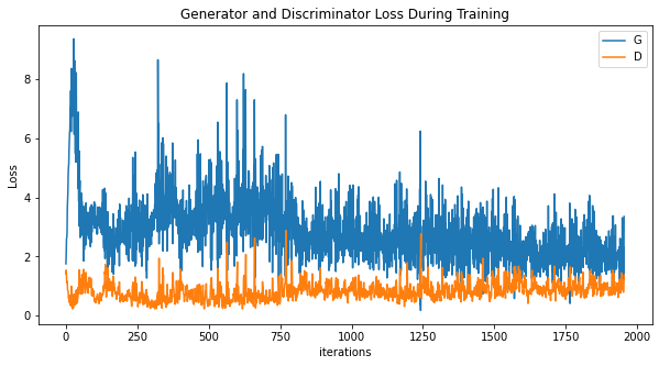
Results#
Let’s train our GAN with current arguments (opt).
We print:
loss values for generator and discriminator.
accuracies of discriminator in detecting real images (x) and fake images (z). In theory, both these numbers start near 1 and should converge to 0.5 (the point where the generator is equally good real and fake images).
generator, d_losses, g_losses, accs_d_x, accs_d_z = train_instance(opt)
Generator(
  (main): Sequential(
    (0): ConvTranspose2d(100, 512, kernel_size=(4, 4), stride=(1, 1), bias=False)
    (1): BatchNorm2d(512, eps=1e-05, momentum=0.1, affine=True, track_running_stats=True)
    (2): ReLU(inplace=True)
    (3): ConvTranspose2d(512, 256, kernel_size=(4, 4), stride=(2, 2), padding=(1, 1), bias=False)
    (4): BatchNorm2d(256, eps=1e-05, momentum=0.1, affine=True, track_running_stats=True)
    (5): ReLU(inplace=True)
    (6): ConvTranspose2d(256, 128, kernel_size=(4, 4), stride=(2, 2), padding=(1, 1), bias=False)
    (7): BatchNorm2d(128, eps=1e-05, momentum=0.1, affine=True, track_running_stats=True)
    (8): ReLU(inplace=True)
    (9): ConvTranspose2d(128, 64, kernel_size=(4, 4), stride=(2, 2), padding=(1, 1), bias=False)
    (10): BatchNorm2d(64, eps=1e-05, momentum=0.1, affine=True, track_running_stats=True)
    (11): ReLU(inplace=True)
    (12): ConvTranspose2d(64, 3, kernel_size=(1, 1), stride=(1, 1), bias=False)
    (13): Tanh()
  )
)
Discriminator(
  (main): Sequential(
    (0): Conv2d(3, 64, kernel_size=(4, 4), stride=(2, 2), padding=(1, 1), bias=False)
    (1): LeakyReLU(negative_slope=0.2, inplace=True)
    (2): Conv2d(64, 128, kernel_size=(4, 4), stride=(2, 2), padding=(1, 1), bias=False)
    (3): BatchNorm2d(128, eps=1e-05, momentum=0.1, affine=True, track_running_stats=True)
    (4): LeakyReLU(negative_slope=0.2, inplace=True)
    (5): Conv2d(128, 256, kernel_size=(4, 4), stride=(2, 2), padding=(1, 1), bias=False)
    (6): BatchNorm2d(256, eps=1e-05, momentum=0.1, affine=True, track_running_stats=True)
    (7): LeakyReLU(negative_slope=0.2, inplace=True)
    (8): Conv2d(256, 512, kernel_size=(4, 4), stride=(2, 2), padding=(1, 1), bias=False)
    (9): BatchNorm2d(512, eps=1e-05, momentum=0.1, affine=True, track_running_stats=True)
    (10): LeakyReLU(negative_slope=0.2, inplace=True)
    (11): Conv2d(512, 1, kernel_size=(2, 2), stride=(1, 1), bias=False)
    (12): Sigmoid()
  )
)
[Epoch 000/5]	[Batch 0000/391]	[G loss: 1.7562]	[D loss: 1.4129 	accs: x=28% 	z=91%]
[Epoch 001/5]	[Batch 0109/391]	[G loss: 3.4918]	[D loss: 0.7350 	accs: x=84% 	z=93%]
[Epoch 002/5]	[Batch 0218/391]	[G loss: 3.3814]	[D loss: 0.7681 	accs: x=83% 	z=92%]
[Epoch 003/5]	[Batch 0327/391]	[G loss: 3.1141]	[D loss: 0.7984 	accs: x=82% 	z=91%]
plt.figure(figsize=(10,5))
plt.title("Generator and Discriminator Loss During Training")
plt.plot(g_losses,label="G")
plt.plot(d_losses,label="D")
plt.xlabel("iterations")
plt.ylabel("Loss")
plt.legend()
plt.show()
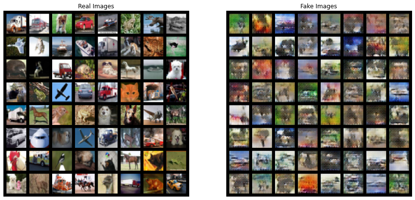
Generating#
# Grab a batch of real images from the dataloader
real_batch = next(iter(dataloader))

# Plot the real images
plt.figure(figsize=(15,15))
plt.subplot(1,2,1)
plt.axis("off")
plt.title("Real Images")
plt.imshow(np.transpose(torchvision.utils.make_grid(real_batch[0].to(device)[:64], padding=5, normalize=True).cpu(),(1,2,0)))


with torch.no_grad():
    gen_imgs = generator(fixed_noise).detach().cpu()

# Plot the fake images from the last epoch
plt.subplot(1,2,2)
plt.axis("off")
plt.title("Fake Images")
plt.imshow(np.transpose(torchvision.utils.make_grid(gen_imgs.to(device)[:64], padding=5, normalize=True).cpu(),(1,2,0)))
plt.show()
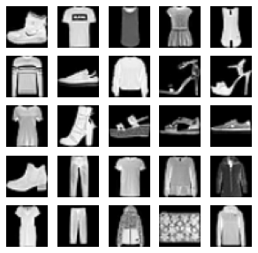
Another dataset#
Let’s play with another dataset!
opt = set_args("--n_epochs", "5", "--dataset", "fashion-mnist")
print(opt)

dataloader = get_dataloader(opt, transform)

fig = plt.figure(figsize=(5, 5))
for i in range(25):
    img, target = dataloader.dataset.__getitem__(i)
    ax = fig.add_subplot(5, 5, i+1)
    ax.imshow(img.numpy().transpose(1, 2, 0) * std + mean, cmap='gray')
    ax.axis('off')
Namespace(n_epochs=5, batch_size=128, lr=0.0002, b1=0.5, b2=0.999, n_cpu=8, latent_dim=100, img_size=32, channels=1, sample_interval=500, out_dir='./gan_out//fashion-mnist/', dataset='fashion-mnist')
generator, d_losses, g_losses, accs_d_x, accs_d_z = train_instance(opt)
Generator(
  (main): Sequential(
    (0): ConvTranspose2d(100, 512, kernel_size=(4, 4), stride=(1, 1), bias=False)
    (1): BatchNorm2d(512, eps=1e-05, momentum=0.1, affine=True, track_running_stats=True)
    (2): ReLU(inplace=True)
    (3): ConvTranspose2d(512, 256, kernel_size=(4, 4), stride=(2, 2), padding=(1, 1), bias=False)
    (4): BatchNorm2d(256, eps=1e-05, momentum=0.1, affine=True, track_running_stats=True)
    (5): ReLU(inplace=True)
    (6): ConvTranspose2d(256, 128, kernel_size=(4, 4), stride=(2, 2), padding=(1, 1), bias=False)
    (7): BatchNorm2d(128, eps=1e-05, momentum=0.1, affine=True, track_running_stats=True)
    (8): ReLU(inplace=True)
    (9): ConvTranspose2d(128, 64, kernel_size=(4, 4), stride=(2, 2), padding=(1, 1), bias=False)
    (10): BatchNorm2d(64, eps=1e-05, momentum=0.1, affine=True, track_running_stats=True)
    (11): ReLU(inplace=True)
    (12): ConvTranspose2d(64, 1, kernel_size=(1, 1), stride=(1, 1), bias=False)
    (13): Tanh()
  )
)
Discriminator(
  (main): Sequential(
    (0): Conv2d(1, 64, kernel_size=(4, 4), stride=(2, 2), padding=(1, 1), bias=False)
    (1): LeakyReLU(negative_slope=0.2, inplace=True)
    (2): Conv2d(64, 128, kernel_size=(4, 4), stride=(2, 2), padding=(1, 1), bias=False)
    (3): BatchNorm2d(128, eps=1e-05, momentum=0.1, affine=True, track_running_stats=True)
    (4): LeakyReLU(negative_slope=0.2, inplace=True)
    (5): Conv2d(128, 256, kernel_size=(4, 4), stride=(2, 2), padding=(1, 1), bias=False)
    (6): BatchNorm2d(256, eps=1e-05, momentum=0.1, affine=True, track_running_stats=True)
    (7): LeakyReLU(negative_slope=0.2, inplace=True)
    (8): Conv2d(256, 512, kernel_size=(4, 4), stride=(2, 2), padding=(1, 1), bias=False)
    (9): BatchNorm2d(512, eps=1e-05, momentum=0.1, affine=True, track_running_stats=True)
    (10): LeakyReLU(negative_slope=0.2, inplace=True)
    (11): Conv2d(512, 1, kernel_size=(2, 2), stride=(1, 1), bias=False)
    (12): Sigmoid()
  )
)
[Epoch 000/5]	[Batch 0000/469]	[G loss: 2.1311]	[D loss: 1.5856 	accs: x=88% 	z=54%]
[Epoch 001/5]	[Batch 0031/469]	[G loss: 3.0232]	[D loss: 0.5454 	accs: x=90% 	z=93%]
[Epoch 002/5]	[Batch 0062/469]	[G loss: 2.7450]	[D loss: 0.5962 	accs: x=89% 	z=92%]
[Epoch 003/5]	[Batch 0093/469]	[G loss: 2.7019]	[D loss: 0.6003 	accs: x=89% 	z=92%]
[Epoch 004/5]	[Batch 0124/469]	[G loss: 2.7537]	[D loss: 0.5892 	accs: x=89% 	z=92%]
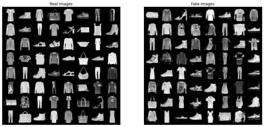
# Grab a batch of real images from the dataloader
real_batch = next(iter(dataloader))

# Plot the real images
plt.figure(figsize=(15,15))
plt.subplot(1,2,1)
plt.axis("off")
plt.title("Real Images")
plt.imshow(np.transpose(torchvision.utils.make_grid(real_batch[0].to(device)[:64], padding=5, normalize=True).cpu(),(1,2,0)))


with torch.no_grad():
    gen_imgs = generator(fixed_noise).detach().cpu()

# Plot the fake images from the last epoch
plt.subplot(1,2,2)
plt.axis("off")
plt.title("Fake Images")
plt.imshow(np.transpose(torchvision.utils.make_grid(gen_imgs.to(device)[:64], padding=5, normalize=True).cpu(),(1,2,0)))
plt.show()