1.3. Pooling

In many networks, it is desirable to gradually reduce the spatial resolution to reach the final output. Pooling is a common operation to achieve this. Similar to convolution pooling is a sliding window operation performing the pooling at all pixels.

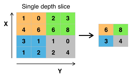
There are two major types of pooling:

• Max the maximum value in the kernel window is the pooled output.

• Average the average of all cells in the kernel window is the pooled output.

0. Preparation

Packages

Let’s start with all the necessary packages to implement this tutorial.

• numpy is the main package for scientific computing with Python. It’s often imported with the np shortcut.

• matplotlib is a library to plot graphs in Python.

• torch is a deep learning framework that allows us to define networks, handle datasets, optimise a loss function, etc.

• skimage is a collection of image processing algorithms.

• request is a simple HTTP library.

# importing the necessary packages/libraries
import numpy as np
from matplotlib import pyplot as plt
import skimage
import torch

Input image

In our example, we work with images to see the effect of convolution on them. First, we read two images by their URL using the skimage.io.imread function. Next, we visualise the images using matplotlibt routines.

# URLs of the images we will load
urls = [
    'https://www2.eecs.berkeley.edu/Research/Projects/CS/vision/bsds/BSDS300/html/images/plain/normal/color/295087.jpg',
    'https://www2.eecs.berkeley.edu/Research/Projects/CS/vision/bsds/BSDS300/html/images/plain/normal/color/35008.jpg'
]

# Load the images using list comprehension
imgs = [skimage.io.imread(url) for url in urls]

# Visualise the two images side by side
fig = plt.figure(figsize=(12, 4))            # Create a figure with a custom size
for img_ind, img in enumerate(imgs):         # Looping through the images
    ax = fig.add_subplot(1, 2, img_ind + 1)  # Add subplots for each image
    ax.imshow(img)                           # Display the image

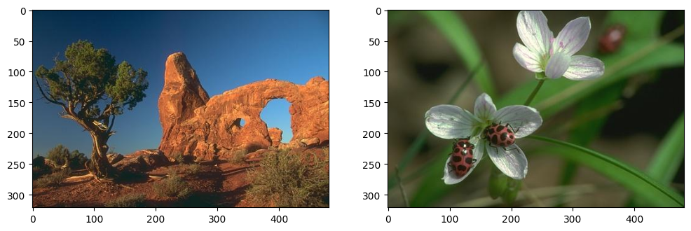
Our input images have spatial resolution \(321 \times 481\).

print("Image size:", imgs[0].shape)

Image size: (321, 481, 3)

Tensor

In this tutorial, we’ll use torch as one of the frameworks that support basic operations.

torch expects images in a different format, the type should be float and channels should proceed the spatial dimension, i.e., (3, w, h).

Furthermore, torch functions are designed for Tensors of 4D, where the first dimension corresponds to different images (b, 3, w, h). In our example, b equals 2 as we have loaded two images.

# converting the images from uint8 to float and create a torch tensor
torch_tensors = [torch.from_numpy(img.astype('float32')) / 255 for img in imgs]
# permuting the tensor to place the RGB channles as the first dimension
torch_tensors = [torch.permute(torch_tensor, (2, 0, 1)) for torch_tensor in torch_tensors]
# stacking both images into one 4D tensor
torch_tensors = torch.stack(torch_tensors, dim=0)
print("Tensor size:", torch_tensors.shape)

Tensor size: torch.Size([2, 3, 321, 481])

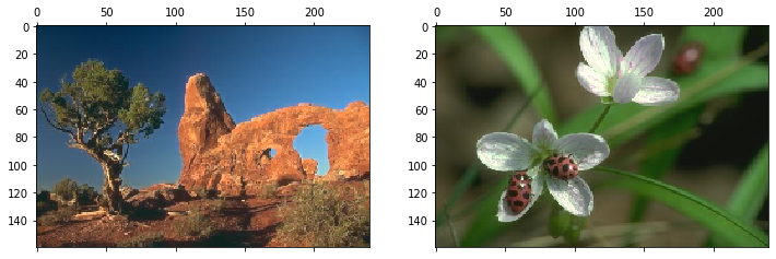
1. Max pooling

Let’s perform max pooling on our input images with kernel_size=(2, 2). We can see the output resolution is halved \(160 \times 240\).

max_pool = torch.nn.MaxPool2d(kernel_size=(2, 2))
max_out = max_pool(torch_tensors)
print(max_out.shape)

torch.Size([2, 3, 160, 240])

max_out_np = max_out.numpy()
max_out_np = np.transpose(max_out_np, (0, 2, 3, 1))

# visualising both images we loaded
fig = plt.figure(figsize=(12, 4))
for img_ind, img in enumerate(max_out_np):
    ax = fig.add_subplot(1, 2, img_ind + 1)
    ax.matshow(img)

Let’s create a small tensor of size \(4 \times 4\) to better understand the output of max pooling.

small_tensor = torch.randint(0, 10, (1, 1, 4, 4)).float()
print(small_tensor.squeeze())

tensor([[6., 9., 9., 2.],
        [6., 9., 6., 0.],
        [8., 3., 4., 5.],
        [9., 2., 3., 5.]])

We can see the output is a \(2 \times 2\) matrix with pooled values corresponding to the maximum values from input pixels.

print(max_pool(small_tensor).squeeze())

tensor([[9., 9.],
        [9., 5.]])

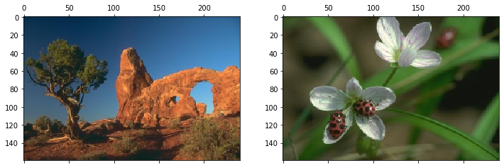
2. Average pooling

Let’s perform average pooling on our input images with kernel_size=(2, 2). We can see the output resolution is halved .

avg_pool = torch.nn.AvgPool2d(kernel_size=(2, 2))
avg_out = avg_pool(torch_tensors)
print(avg_out.shape)

torch.Size([2, 3, 160, 240])

avg_out_np = avg_out.numpy()
avg_out_np = np.transpose(avg_out_np, (0, 2, 3, 1))

# visualising both images we loaded
fig = plt.figure(figsize=(12, 4))
for img_ind, img in enumerate(avg_out_np):
    ax = fig.add_subplot(1, 2, img_ind + 1)
    ax.matshow(img)

Let’s compute the average pooling overrour small tensor of size \(4 \times 4\).

We can see the output is a \(2 \times 2\) matrix with pooled values corresponding to the average values from input pixels.

print(avg_pool(small_tensor).squeeze())

tensor([[7.5000, 4.2500],
        [5.5000, 4.2500]])

3. Max versus average pooling

If we compare the output of max and average pooling over the small tensor, we can see big differences:

• In the case of max pooling, three out of four pixels have the same value (9).

• The very same pixels, in average pooling result in three different numbers.

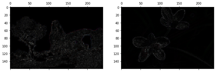
Let’s visualise the difference in natural images:

# visualising both images we loaded
fig = plt.figure(figsize=(12, 4))
for img_ind, img in enumerate(avg_out_np):
    ax = fig.add_subplot(1, 2, img_ind + 1)
    ax.matshow(abs(img - max_out_np[img_ind]))

4. Global pooling

Pooling layers reduce the spatial size of feature maps.

• With normal pooling (e.g., AvgPool2d, MaxPool2d), we specify the window size.

• With global pooling, we specify the output size. This makes global pooling especially useful before fully connected layers, as it converts any feature map into a fixed-size vector.

Let’s create a small tensor of size \(4 \times 4\) to better understand the difference.

# Create a simple 4×4 feature map
x = torch.tensor([[[[1., 2., 3., 4.],
                    [5., 6., 7., 8.],
                    [9.,10.,11.,12.],
                    [13.,14.,15.,16.]]]])

print("Input shape:", x.shape)
print(x)

Input shape: torch.Size([1, 1, 4, 4])
tensor([[[[ 1.,  2.,  3.,  4.],
          [ 5.,  6.,  7.,  8.],
          [ 9., 10., 11., 12.],
          [13., 14., 15., 16.]]]])

# Normal pooling: specify window size
avg_pool = torch.nn.AvgPool2d(kernel_size=2)
max_pool = torch.nn.MaxPool2d(kernel_size=2)

avg_out = avg_pool(x)
max_out = max_pool(x)

print("\nAverage Pooling (2×2 window):")
print(avg_out)

print("\nMax Pooling (2×2 window):")
print(max_out)

Average Pooling (2×2 window):
tensor([[[[ 3.5000,  5.5000],
          [11.5000, 13.5000]]]])

Max Pooling (2×2 window):
tensor([[[[ 6.,  8.],
          [14., 16.]]]])

# Global pooling: specify output size
global_avg = torch.nn.AdaptiveAvgPool2d(output_size=(1, 1))
global_max = torch.nn.AdaptiveMaxPool2d(output_size=(1, 1))

gavg_out = global_avg(x)
gmax_out = global_max(x)

print("\nGlobal Average Pooling (output size = 1×1):")
print(gavg_out)

print("\nGlobal Max Pooling (output size = 1×1):")
print(gmax_out)

Global Average Pooling (output size = 1×1):
tensor([[[[8.5000]]]])

Global Max Pooling (output size = 1×1):
tensor([[[[16.]]]])