5.3. Language – Vision#
In this notebook, we will learn how to train a multimodal network. We will explore a language–vision model which matches texts to images. In particular, we implement a simple CLIP (Contrastive Language-Image Pre-Training).
CLIP is a neural network trained on various (image, text) pairs. It can be instructed in natural language to predict the most relevant text snippet, given an image, without directly optimizing for the task, similar to the zero-shot capabilities of GPT-2 and 3.

0. Preparation#
In order to run this notebook, we need to perform some preparations.
Packages#
Let’s start with all the necessary packages to implement this tutorial.
numpy is the main package for scientific computing with Python. It’s often imported with the
npshortcut.os provides a portable way of using operating system-dependent functionality, e.g., modifying files/folders.
pandas provides easy working routines with tabular data structures.
argparse is a module making it easy to write user-friendly command-line interfaces.
matplotlib is a library to plot graphs in Python.
torch is a deep learning framework that allows us to define networks, handle datasets, optimise a loss function, etc.
transformers provides pretrained models to perform tasks on different modalities such as text, vision, and audio.
import numpy as np
import os
import pandas as pd
import argparse
import itertools

import matplotlib.pyplot as plt
from PIL import Image as pil_image

import torch
from torch import nn
import torchvision

from transformers import DistilBertModel, DistilBertTokenizer
device#
Choosing CPU or GPU based on the availability of the hardware.
device = torch.device('cuda' if torch.cuda.is_available() else 'cpu')
arguments#
We use the argparse module to define a set of parameters that we use throughout this notebook:
The
argparseis particularly useful when writing Python scripts, allowing you to run the same script with different parameters (e.g., for doing different experiments).In notebooks using
argparseis not necessarily beneficial, we could have hard-coded those values directly in variables, but here we useargparsefor learning purposes.
parser = argparse.ArgumentParser()
parser.add_argument("--epochs", type=int, default=5, help="number of training epochs")
parser.add_argument("--batch_size", type=int, default=8, help="size of the batches")
parser.add_argument("--num_workers", type=int, default=0, help="number of CPU workers")

parser.add_argument("--head_lr", type=float, default=1e-3, help="Head learning rate")
parser.add_argument("--image_encoder_lr", type=float, default=1e-4, help="Image encoder learning rate")
parser.add_argument("--text_encoder_lr", type=float, default=1e-5, help="Text encoder learning rate")
parser.add_argument("--weight_decay", type=float, default=1e-3, help="Weight decay")
parser.add_argument("--projection_dim", type=float, default=256, help="Size of the projection space")

parser.add_argument("--model_vision", type=str, default='resnet50', help="Image encoder")
parser.add_argument("--model_text", type=str, default='distilbert-base-uncased', help="Text encoder")

parser.add_argument("--img_size", type=int, default=224, help="size of each image dimension")
parser.add_argument("--log_frequency", type=int, default=100, help="interval log prints")
parser.add_argument("--out_dir", type=str, default="./out/clip_out/", help="the output directory")
parser.add_argument("--data_dir", type=str, default="./data/", help="the dataset directory")

def set_args(*args):
    # we can pass arguments to the parse_args function to change the default values.
    opt = parser.parse_args([*args])
    # creating the output directory
    os.makedirs(opt.out_dir, exist_ok=True)
    return opt
1. Datasets#
We have created the TinyFlicker dataset which is a subset of Flickr8k dataset. The TinyFlicker contains:
1000 images,
5 captions per image.
Download and extract#
The download_and_extract_db function downloads and extracts the dataset if it’s not already
stored in the provided directory. We use two functions already implemented in torchvision.datasets.utils:
download_urlextract_archive
def download_and_extract_db(data_dir):
    db_url = "https://dl.dropboxusercontent.com/s/zi46giyvvch0k8q/TinyFlicker.tar.gz"
    torchvision.datasets.utils.download_url(db_url, data_dir)

    data_dir = torchvision.datasets.utils.extract_archive(
        "%s/TinyFlicker.tar.gz" % data_dir, "%s/TinyFlicker/" % data_dir
    )
    return data_dir
Text Tokeniser#
We could have created our own text tokeniser similar to the text classification notebook.
But in this tutorial, we use DistilBertTokenizer from the transformers package.
text_tokeniser = DistilBertTokenizer.from_pretrained("distilbert-base-uncased")
Dataset class#
The TinyFlicker class reads the dataset file and returns the pair of image-caption.
class TinyFlicker(torch.utils.data.Dataset):
    def __init__(self, root, data_frame, tokeniser, transforms=None, max_tokens=50):
        self.root = root
        self.captions = data_frame['caption'].values
        self.images = data_frame['image'].values
        self.tokeniser = tokeniser
        self.transforms = transforms
        self.max_tokens = max_tokens

    def __getitem__(self, idx):
        # loading the image
        img = pil_image.open("%s/imgs/%s" % (self.root, self.images[idx]))
        # performing the transformation functions
        if self.transforms:
            img = self.transforms(img)
        caption = self.captions[idx]

        # tokenising the text
        tout = self.tokeniser(caption, truncation=True, max_length=self.max_tokens)
        input_ids = torch.tensor(tout['input_ids'])
        attention_mask = torch.tensor(tout['attention_mask'])
        # all elements in each batch should have the same length, therefore we pad
        # the tensors into an identical length
        input_ids = nn.functional.pad(input_ids, (0, self.max_tokens - len(input_ids)), value=0)
        attention_mask = nn.functional.pad(attention_mask, (0, self.max_tokens - len(attention_mask)), value=0)

        item = {
            'image': img,
            'caption': caption,
            'input_ids': input_ids,
            'attention_mask': attention_mask
        }
        return item

    def __len__(self):
        return len(self.captions)
Transform functions#
In this tutorial, we use the same set of transform functions for training and testing. Essentially, we only resize the input images and convert them to a normalised tensor. One could add data augmentation to the training images such as random cropping or horizontal flipping. We leave this as an exercise for interested readers.
def get_transforms(target_size, for_network=True):
    mean = [0.485, 0.456, 0.406]
    std = [0.229, 0.224, 0.225]
    transform_funs = [
        torchvision.transforms.Resize(target_size),
        torchvision.transforms.CenterCrop(target_size)
    ]
    # if for_networks is False we don't convert it to Tensor and normalisation. This
    # makes it easier for visualisation purposes.
    if for_network:
        transform_funs.extend([
            torchvision.transforms.ToTensor(),
            torchvision.transforms.Normalize(mean, std)
        ])
    return torchvision.transforms.Compose(transform_funs)
Sample items#
Let’s create an instance of our dataset and explore its content. The first time you execute the
the following cell, it downloads the dataset and extracts its content in the data_dir directory.
data_dir = './data/'
data_dir = download_and_extract_db(data_dir)
data_frame = pd.read_csv("%s/captions.csv" % data_dir)
sample_db = TinyFlicker(
    root=data_dir,
    data_frame=data_frame,
    tokeniser=text_tokeniser,
    transforms=get_transforms(224, for_network=False),
)
Using downloaded and verified file: ./data/TinyFlicker.tar.gz
print('The number of samples in the dataset: %d' % sample_db.__len__())
The number of samples in the dataset: 5000
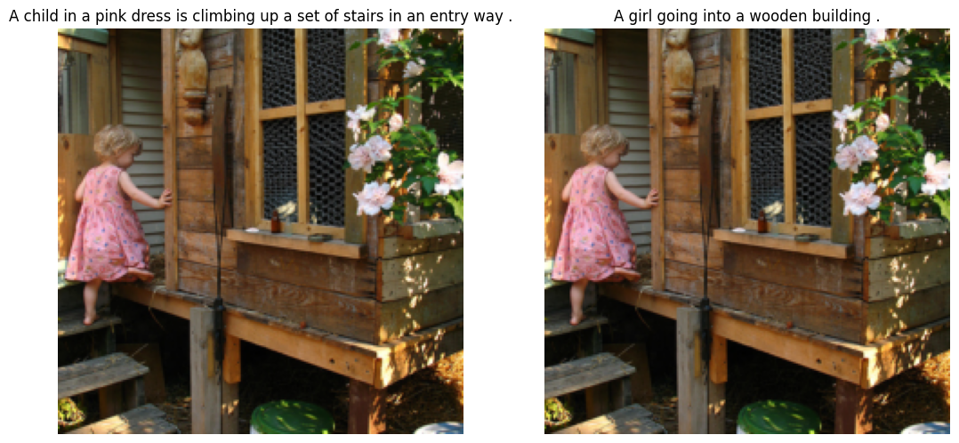
Each sample is a dict of four elements:
image: the input image
caption: the raw image caption
input_ids: the processed caption by
text_tokeniserattention_mask: an array of 1s and 0s corresponding to actual text or padded zeros.
sample_item = sample_db.__getitem__(0)
print(sample_item.keys())
dict_keys(['image', 'caption', 'input_ids', 'attention_mask'])
If we print the input_ids each cell corresponds to index of that word (token) in the dictionary.
Please check the text classification notebook for more information.
sample_item['input_ids']
tensor([ 101, 1037, 2775, 1999, 1037, 5061, 4377, 2003, 8218, 2039, 1037, 2275,
        1997, 5108, 1999, 2019, 4443, 2126, 1012,  102,    0,    0,    0,    0,
           0,    0,    0,    0,    0,    0,    0,    0,    0,    0,    0,    0,
           0,    0,    0,    0,    0,    0,    0,    0,    0,    0,    0,    0,
           0,    0])
The attention_mask tensor have the same length as input_ids:
Those with value 1 correspond to actual word (token)
Those with value 0 are padded element.
print('Size of input_ids:', sample_item['input_ids'].shape)
print('Size of attention_mask:', sample_item['attention_mask'].shape)
sample_item['attention_mask']
Size of input_ids: torch.Size([50])
Size of attention_mask: torch.Size([50])
tensor([1, 1, 1, 1, 1, 1, 1, 1, 1, 1, 1, 1, 1, 1, 1, 1, 1, 1, 1, 1, 0, 0, 0, 0,
        0, 0, 0, 0, 0, 0, 0, 0, 0, 0, 0, 0, 0, 0, 0, 0, 0, 0, 0, 0, 0, 0, 0, 0,
        0, 0])
Let’s plot two captions for an identical image:
fig = plt.figure(figsize=(20, 6))
for i in range(2):
    sample_item = sample_db.__getitem__(i)
    ax = fig.add_subplot(1, 3, i+1)
    ax.imshow(sample_item['image'])
    ax.axis('off')
    ax.set_title(sample_item['caption'], wrap=True)
Dataloaders#
We make standard 80-20% train/test splits.
def make_train_valid_dfs(data_dir, val_percent=0.2):
    dataframe = pd.read_csv("%s/captions.csv" % data_dir)
    dataframe['id'] = [id_ for id_ in range(dataframe.shape[0] // 5) for _ in range(5)]
    max_id = dataframe["id"].max() + 1
    image_ids = np.arange(0, max_id)
    valid_ids = np.random.choice(image_ids, size=int(val_percent * len(image_ids)), replace=False)
    train_ids = [id_ for id_ in image_ids if id_ not in valid_ids]
    train_dataframe = dataframe[dataframe["id"].isin(train_ids)].reset_index(drop=True)
    valid_dataframe = dataframe[dataframe["id"].isin(valid_ids)].reset_index(drop=True)
    return train_dataframe, valid_dataframe

def build_loaders(args, data_frame, mode):
    transforms = get_transforms(args.img_size)
    dataset = TinyFlicker(
        root=args.data_dir,
        data_frame=data_frame,
        tokeniser=text_tokeniser,
        transforms=transforms,
    )
    dataloader = torch.utils.data.DataLoader(
        dataset,
        batch_size=args.batch_size,
        num_workers=args.num_workers,
        shuffle=True if mode == "train" else False,
    )
    return dataloader
2. Network#
The CLIP Network consists of three main parts:
Image encoder that encodes the visual signal. In theory, it can be any architecture (pretrained network). The only requirement is to have the output as a flattened vector.
Text encoder that encodes the text data. Similar to the image encoder, the text encoder can be any architecture.
CLIPNet projects the image/text embeddings into a common embedding space and computes their similarity using matrix multiplication.
Vision#
We have hard-coded our ImageEncoder to the last layer of a ResNet50 pretrained on ImageNet.
In our case, the output of ImageEncoder is a vector of size 2048.
Interested readers can change the code to support different image encoders.
# Encoder for processing images
class ImageEncoder(nn.Module):
    def __init__(self, model_name):
        super().__init__()
        # Load a pre-trained ResNet-50 model (using ImageNet weights) and remove the final classification layer
        pretrained = torchvision.models.resnet50(weights=torchvision.models.ResNet50_Weights.IMAGENET1K_V2)
        self.model = nn.Sequential(*list(pretrained.children())[:-1])
        # Set the dimensionality of the output embeddings from the encoder
        self.embedding_dim = 2048

    def forward(self, x):
        # Pass the image through the ResNet-50 model
        x = self.model(x)
        # Flatten the output to a 2D tensor (batch_size, embedding_dim)
        return torch.flatten(x, start_dim=1)
Language#
We have hard-coded our TextEncoder to the last layer of a DistilBertModel which is a
transformer-based model for natural language processing (NLP) tasks. We use its implementation
from the transformers package. We use the transformers package instead of torchtext because
it does not have many powerful pretrained text models.
In our case, the output of TextEncoder is a vector of size 768.
Interested readers can change the code to support different text encoders.
# Encoder for processing text
class TextEncoder(nn.Module):
    def __init__(self, model_name):
        super().__init__()
        # Load a pre-trained DistilBERT model from the HuggingFace Transformers library
        self.model = DistilBertModel.from_pretrained(model_name)
        # Set the dimensionality of the output embeddings from the encoder
        self.embedding_dim = 768
        # Use the [CLS] token (index 0) as the representation of the whole input text
        self.target_token_idx = 0

    def forward(self, input_ids, attention_mask):
        # Pass the text through the DistilBERT model
        output = self.model(input_ids=input_ids, attention_mask=attention_mask)
        last_hidden_state = output.last_hidden_state
        # Extract the embedding of the [CLS] token
        return last_hidden_state[:, self.target_token_idx, :]
CLIP Network#
The ProjectionHead brings the image/text embedding vectors from their corresponding dimensions
(in our case 2048 and 768 respectively) to a common projection space (in our case 256).
The CLIPNet combines all the above-mentioned building blocks into one network:
Encoding text.
Encoding image.
Projecting text features into the common space.
Projecting image features into the common space.
Computing the similarity by doing matrix multiplication (@ operation) between the projected image/text embeddings.
# A projection head to map encoder outputs to a shared embedding space
class ProjectionHead(nn.Module):
    def __init__(self, embedding_dim, projection_dim):
        super().__init__()
        # Linear layer to project the encoder's output to a lower-dimensional space
        self.projection = nn.Linear(embedding_dim, projection_dim)
        self.gelu = nn.GELU()  # Activation function
        self.fc = nn.Linear(projection_dim, projection_dim)  # Fully connected layer
        self.layer_norm = nn.LayerNorm(projection_dim)  # Normalize embeddings

    def forward(self, x):
        # Project the input embeddings
        projected = self.projection(x)
        # Apply activation and a second linear layer
        x = self.gelu(projected)
        x = self.fc(x)
        # Add skip connection and normalize
        x = x + projected
        x = self.layer_norm(x)
        return x
# The main CLIP model combining image and text encoders
class CLIPNet(nn.Module):
    def __init__(self, vision_model_name, text_model_name, projection_dim):
        super().__init__()
        # Initialize the image and text encoders
        self.image_encoder = ImageEncoder(vision_model_name)
        self.text_encoder = TextEncoder(text_model_name)
        # Add projection heads to map encoder outputs to a common embedding space
        self.image_projection = ProjectionHead(self.image_encoder.embedding_dim, projection_dim)
        self.text_projection = ProjectionHead(self.text_encoder.embedding_dim, projection_dim)

    def forward(self, batch):
        # Process text inputs to obtain text features
        text_features = self.text_encoder(
            input_ids=batch["input_ids"], attention_mask=batch["attention_mask"]
        )
        # Process image inputs to obtain image features
        image_features = self.image_encoder(batch["image"])
        # Project features into the shared embedding space
        text_embeddings = self.text_projection(text_features)
        image_embeddings = self.image_projection(image_features)

        # Compute similarity scores between text and image embeddings
        logits = text_embeddings @ image_embeddings.T
        # Compute self-similarity matrices for images and texts
        image_similarity = image_embeddings @ image_embeddings.T
        text_similarity = text_embeddings @ text_embeddings.T

        # Generate targets by averaging image and text similarities
        targets = torch.softmax((image_similarity + text_similarity) / 2, dim=-1)

        # Compute cross-entropy loss for both directions
        text_loss = nn.functional.cross_entropy(logits, targets, reduction='none')
        image_loss = nn.functional.cross_entropy(logits.T, targets.T, reduction='none')

        # Average the two losses to ensure bidirectional alignment
        loss = (image_loss + text_loss) / 2.0  # shape: (batch_size)

        # Return the mean loss over the batch
        return loss.mean()
In the best theoretical scenario, text_embeddings and image_embedding matrices should be the same
(or highly correlated) because they are describing similar things. If this happens, what would the
logits matrix look like? Let’s see with a simple example!
The target (matched image-text pairs) becomes a diagonal matrix.
batch_size = 4
dim = 256
embeddings = torch.randn(batch_size, dim)
out = embeddings @ embeddings.T
target = torch.softmax(out, dim=-1)
print(target)
tensor([[1., 0., 0., 0.],
        [0., 1., 0., 0.],
        [0., 0., 1., 0.],
        [0., 0., 0., 1.]])
3. Train/test routines#
The following routines are very similar (close to identical) to what we previously saw in the image classification problem.
def epoch_loop(model, dataloader, optimiser, log_frequency=100):
    # usually the code for train/test has a large overlap.
    is_train = False if optimiser is None else True

    # model should be in train/eval model accordingly
    model.train() if is_train else model.eval()

    losses = []
    with torch.set_grad_enabled(is_train):
        for batch_ind, batch in enumerate(dataloader):
            batch = {k: v.to(device) for k, v in batch.items() if k != "caption"}
            loss = model(batch)
            losses.extend([loss.item() for _ in range(batch["image"].size(0))])

            if batch_ind % log_frequency == 0 and batch_ind > 0:
                print(
                    '%s batches [%.5d/%.5d] \tloss=%.4f' % (
                        'training' if is_train else 'testing', batch_ind,
                        len(dataloader), np.mean(losses)
                    )
                )

            if is_train:
                optimiser.zero_grad()
                loss.backward()
                optimiser.step()
    return losses
def main(args):
    args.data_dir = download_and_extract_db(args.data_dir)
    train_df, valid_df = make_train_valid_dfs(args.data_dir)
    train_loader = build_loaders(args, train_df, mode="train")
    valid_loader = build_loaders(args, valid_df, mode="valid")

    model = CLIPNet(args.model_vision, args.model_text, args.projection_dim)
    model = model.to(device)
    params = [
        {"params": model.image_encoder.parameters(), "lr": args.image_encoder_lr},
        {"params": model.text_encoder.parameters(), "lr": args.text_encoder_lr},
        {"params": itertools.chain(
            model.image_projection.parameters(), model.text_projection.parameters()
        ), "lr": args.head_lr, "weight_decay": args.weight_decay}
    ]
    optimizer = torch.optim.AdamW(params, weight_decay=0.)

    logs = {'train': [], 'val': []}
    for epoch in range(args.epochs):
        print("Epoch: [%.3d/%.3d]" % (epoch, args.epochs))
        model.train()
        train_loss = epoch_loop(model, train_loader, optimizer, args.log_frequency)
        logs['train'].append(np.mean(train_loss))
        valid_loss = epoch_loop(model, valid_loader, None)
        logs['val'].append(np.mean(valid_loss))

        print('Train     loss=%.4f     Test     loss=%.4f' %
              (np.mean(train_loss), np.mean(valid_loss)))
        # saving the checkpoint
        torch.save(model.state_dict(), "%s/checkpoint.pth.tar" % args.out_dir)
    return logs
Let’s train our network for ten epochs:
args = set_args("--epochs", "10", "--data_dir", "./data/")
print(args)
logs = main(args)
Namespace(epochs=10, batch_size=8, num_workers=0, head_lr=0.001, image_encoder_lr=0.0001, text_encoder_lr=1e-05, weight_decay=0.001, projection_dim=256, model_vision='resnet50', model_text='distilbert-base-uncased', img_size=224, log_frequency=100, out_dir='./out/clip_out/', data_dir='./data/')
Using downloaded and verified file: ./data/TinyFlicker.tar.gz
Epoch: [000/010]
training batches [00100/00625] 	loss=4.4483
training batches [00200/00625] 	loss=3.0828
training batches [00300/00625] 	loss=2.4970
training batches [00400/00625] 	loss=2.1279
training batches [00500/00625] 	loss=1.8743
training batches [00600/00625] 	loss=1.6705
testing batches [00100/00125] 	loss=1.7055
Train     loss=1.6304     Test     loss=1.6853
Epoch: [001/010]
training batches [00100/00625] 	loss=0.4974
training batches [00200/00625] 	loss=0.4904
training batches [00300/00625] 	loss=0.4870
training batches [00400/00625] 	loss=0.4528
training batches [00500/00625] 	loss=0.4569
training batches [00600/00625] 	loss=0.4458
testing batches [00100/00125] 	loss=1.5938
Train     loss=0.4388     Test     loss=1.5842
Epoch: [002/010]
training batches [00100/00625] 	loss=0.2457
training batches [00200/00625] 	loss=0.2380
training batches [00300/00625] 	loss=0.2512
training batches [00400/00625] 	loss=0.2662
training batches [00500/00625] 	loss=0.2629
training batches [00600/00625] 	loss=0.2625
testing batches [00100/00125] 	loss=1.6866
Train     loss=0.2675     Test     loss=1.6693
Epoch: [003/010]
training batches [00100/00625] 	loss=0.2246
training batches [00200/00625] 	loss=0.2256
training batches [00300/00625] 	loss=0.2126
training batches [00400/00625] 	loss=0.2097
training batches [00500/00625] 	loss=0.2076
training batches [00600/00625] 	loss=0.2052
testing batches [00100/00125] 	loss=1.6065
Train     loss=0.2036     Test     loss=1.6124
Epoch: [004/010]
training batches [00100/00625] 	loss=0.2084
training batches [00200/00625] 	loss=0.1841
training batches [00300/00625] 	loss=0.1906
training batches [00400/00625] 	loss=0.1936
training batches [00500/00625] 	loss=0.2045
training batches [00600/00625] 	loss=0.2002
testing batches [00100/00125] 	loss=1.6642
Train     loss=0.2001     Test     loss=1.6516
Epoch: [005/010]
training batches [00100/00625] 	loss=0.1418
training batches [00200/00625] 	loss=0.1478
training batches [00300/00625] 	loss=0.1571
training batches [00400/00625] 	loss=0.1493
training batches [00500/00625] 	loss=0.1562
training batches [00600/00625] 	loss=0.1827
testing batches [00100/00125] 	loss=1.6275
Train     loss=0.1817     Test     loss=1.6241
Epoch: [006/010]
training batches [00100/00625] 	loss=0.1259
training batches [00200/00625] 	loss=0.1453
training batches [00300/00625] 	loss=0.1402
training batches [00400/00625] 	loss=0.1421
training batches [00500/00625] 	loss=0.1480
training batches [00600/00625] 	loss=0.1507
testing batches [00100/00125] 	loss=1.6815
Train     loss=0.1496     Test     loss=1.6759
Epoch: [007/010]
training batches [00100/00625] 	loss=0.1502
training batches [00200/00625] 	loss=0.1629
training batches [00300/00625] 	loss=0.1629
training batches [00400/00625] 	loss=0.1503
training batches [00500/00625] 	loss=0.1487
training batches [00600/00625] 	loss=0.1472
testing batches [00100/00125] 	loss=1.6893
Train     loss=0.1465     Test     loss=1.6839
Epoch: [008/010]
training batches [00100/00625] 	loss=0.1398
training batches [00200/00625] 	loss=0.1192
training batches [00300/00625] 	loss=0.1338
training batches [00400/00625] 	loss=0.1354
training batches [00500/00625] 	loss=0.1361
training batches [00600/00625] 	loss=0.1351
testing batches [00100/00125] 	loss=1.6247
Train     loss=0.1373     Test     loss=1.6101
Epoch: [009/010]
training batches [00100/00625] 	loss=0.1043
training batches [00200/00625] 	loss=0.1097
training batches [00300/00625] 	loss=0.1204
training batches [00400/00625] 	loss=0.1182
training batches [00500/00625] 	loss=0.1214
training batches [00600/00625] 	loss=0.1241
testing batches [00100/00125] 	loss=1.6235
Train     loss=0.1261     Test     loss=1.6347
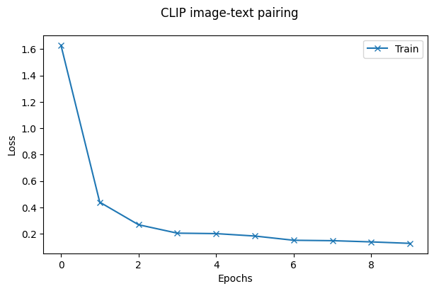
Training progress#
Let’s plot the evolution of loss for both train and test sets.
fig = plt.figure(figsize=(7, 4))
fig.suptitle('CLIP image-text pairing')
ax = fig.add_subplot(1, 1, 1)
ax.plot(np.array(logs['train']), '-x', label="Train")
ax.plot(np.array(logs['val']), '-x', label="Test")
ax.set_xlabel("Epochs")
ax.set_ylabel("Loss")
ax.legend()
<matplotlib.legend.Legend at 0x7a3da2b18d90>
Prediction#
Now we have a model that matches any pairs of image-texts. We can use it for zero-short evaluation in several applications. In this tutorial, we use it for query matching.
Query matching#
The get_image_embeddings function:
Loads the model we have trained
Computed the
image_embeddingsfor all images in the validation set and stored it in a list.We use the list of
image_embeddingslater on for query matching.
def get_image_embeddings(valid_df, model_path):
    valid_loader = build_loaders(args, valid_df, mode="valid")

    model = CLIPNet(args.model_vision, args.model_text, args.projection_dim).to(device)
    model.load_state_dict(torch.load(model_path, map_location=device))
    model.eval()

    valid_image_embeddings = []
    with torch.no_grad():
        for batch in valid_loader:
            image_features = model.image_encoder(batch["image"].to(device))
            image_embeddings = model.image_projection(image_features)
            valid_image_embeddings.append(image_embeddings)
    return model, torch.cat(valid_image_embeddings)
_, valid_df = make_train_valid_dfs(args.data_dir)
model, image_embeddings = get_image_embeddings(valid_df, "%s/checkpoint.pth.tar" % args.out_dir)
Some weights of the model checkpoint at distilbert-base-uncased were not used when initializing DistilBertModel: ['vocab_layer_norm.weight', 'vocab_projector.bias', 'vocab_layer_norm.bias', 'vocab_transform.bias', 'vocab_transform.weight']
- This IS expected if you are initializing DistilBertModel from the checkpoint of a model trained on another task or with another architecture (e.g. initializing a BertForSequenceClassification model from a BertForPreTraining model).
- This IS NOT expected if you are initializing DistilBertModel from the checkpoint of a model that you expect to be exactly identical (initializing a BertForSequenceClassification model from a BertForSequenceClassification model).
The find_matches function searches in all image_embeddings and find those
that best match the passed query argument.
def find_matches(model, image_embeddings, query, image_filenames, n=3):
    encoded_query = text_tokeniser([query])
    batch = {
        key: torch.tensor(values).to(device)
        for key, values in encoded_query.items()
    }
    with torch.no_grad():
        text_features = model.text_encoder(
            input_ids=batch["input_ids"], attention_mask=batch["attention_mask"]
        )
        text_embeddings = model.text_projection(text_features)

    image_embeddings_n = nn.functional.normalize(image_embeddings, p=2, dim=-1)
    text_embeddings_n = nn.functional.normalize(text_embeddings, p=2, dim=-1)
    dot_similarity = text_embeddings_n @ image_embeddings_n.T

    values, indices = torch.topk(dot_similarity.squeeze(0), n * 5)
    matches = [image_filenames[idx] for idx in indices[::5]]

    transforms = get_transforms(args.img_size, for_network=False)
    fig, axes = plt.subplots(1, 3, figsize=(9, 3))
    for match, ax in zip(matches, axes.flatten()):
        image = pil_image.open("%s/imgs/%s" % (args.data_dir, match))
        image = transforms(image)
        ax.imshow(image)
        ax.axis("off")
    fig.suptitle('Query: %s' % query)
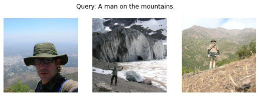
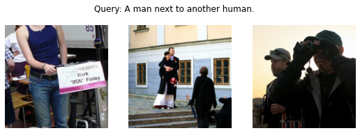
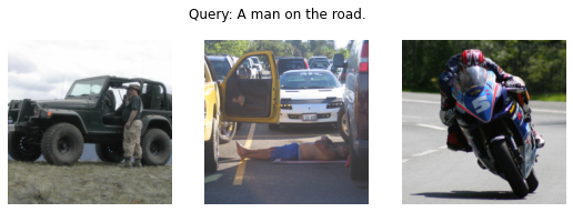
Let’s try our network with three similar phrases to evaluate how well it can distinguish sutle differences:
“A man on the mountains.”
“A man next to another human.”
“A man on the road.”
find_matches(
    model, image_embeddings, image_filenames=valid_df['image'].values,
    query="A man on the mountains."
)
find_matches(
    model, image_embeddings, image_filenames=valid_df['image'].values,
    query="A man next to another human."
)
find_matches(
    model, image_embeddings, image_filenames=valid_df['image'].values,
    query="A man on the road."
)
Excercises#
Below is a list of exercises to practice what we have learnt in this notebook:
Change the vision encoder from ResNet to another network, e.g. ViT.
Plot the query matching results before any training and after each epoch. How fast do the results become qualitatively acceptable?
Train the network without using the pretrained weights.
Add data augmentation to the training pipeline (both for images and captions).
References#
The following sources inspire the materials in this notebook:
